Usage+Spend Forecasting on AWS with FinOps Foundation’s Best Practices

Forecasting is the process of making predictions based on our assumptions about the factors driving the data of interest and its actual past and present values. The key value of having accurate forecasts is that they allow to be proactive, rather than reactive.

In 2020, for one in three respondents, cloud spend was projected to be over budget by between 20 percent and 40 percent. One in 12 respondents said their cloud spend was expected to be over budget by more than 40 percent.

– Pepperdata

Making wrong or no forecasts has a high cost for your Company. Many have wondered if it’s a good idea to forecast at all. In our experience, the answer is yes. While nobody owns a crystal ball, a conservative forecasting model prevents the damage from wild guesses, that, if you don’t build a good model, your team will still implicitly make irrespective on their opinion that forecasts were a bad idea or look at someone else’s model. There is no discussion about this, we saw it happen in small and large Companies.

In the AWS context, we recommend forecasting both usage and spend

• accurate usage forecasts allow, for example,
  • to purchase the right number of reserved instances / savings plans
  • to accurately decide the EC2 / RDS instance type and whether to use serverless instead
  • to accurately set up AWS services parameters
• accurate cost forecasts allow, for example,
  • to create realistic budgets and thus better allocate resources – such as time, money, hiring etc.
  • to help with the solution pricing
  • to determine the cost-effective technology given the expected revenue.

1. AWS Usage Forecasting

We recommend dumping CloudWatch metrics into an S3 data lake using AWS CloudWatch Metric Streams. The setup is well described in this article – choose only the metrics relevant for your forecasting, being aware of the pricing.

The CloudWatch data lake can be also queried with AWS Athena to provide data to answer complex questions, such as identification of usage patterns of EBS drives to optimize their size or their storage class, or quantification of the costs of overprovisioned and unused EC2 instances.

Using AWS CloudWatch Streams is far more powerful than using CloudWatch Metrics Insights, since the latter’s queries are per account only and do not support linked accounts.

1.1. Best Practices for Usage Forecasting

1. Aggregate the usage data across related services – e.g., compute, storage, data transfer
2. Choose the right binning – daily / weekly / monthly data
3. Normalize all data per business-driven unit, such as per customer, or transaction.
4. Use any of the AWS services described below for producing the forecasts

2. AWS Cost Forecasting

We recommend forecasting both net unblended costs and net amortized costs (net indicates they include all discounts):

• net unblended costs – these are the costs as they are charged to you → the costs which show up on your AWS bill → cash basis of accounting
• net amortized costs – these are the effective daily costs, considering all purchased reserved instances and savings plans → accrual basis of accounting.

The best way to illustrate the difference between the net unblended and net amortized costs is to compare them on the day when you purchase a one-year reserved EC2 instance for $X:

1. the net unblended costs jump by $X and the next day there will be no charge for the reserved instance
2. the net amortized costs jump by $X/100 for the next 365 days since the reserved EC2 instance costs are spread over the lifetime of the reserved instance.

2.1. Setting up AWS CUR S3 Data Lake

All below analysis is based upon Cost and Usage Report (CUR) S3 data lake which can be queried by AWS Athena.

To set it up, use the steps described in this document or in the AWS Well Architected Labs.

You can ask AWS via a support request to backfill the CUR S3 bucket for up to 1 year back.

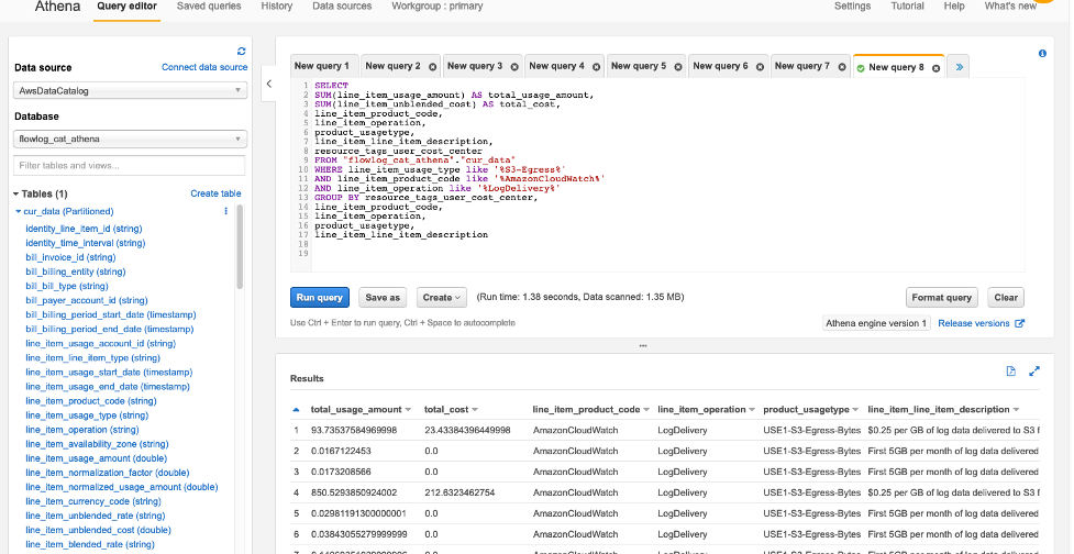
2.2. AWS Athena Query for Net Unblended Costs and Net Amortized Costs

To the best of our knowledge, this is the most accurate Athena query for net unblended and net amortized costs. Notice, the query does differ from AWS Well-Architected Labs’s recommended amortized costs query – our query does reconcile far more accurately with the actual AWS invoice and the AWS Cost Explorer’s Net Amortized costs.

SELECT
      DATE_FORMAT((bill_billing_period_start_date),'%Y-%m-01') AS month_bill_billing_period_start_date, 
      round(SUM(COALESCE(line_item_net_unblended_cost, line_item_unblended_cost)),2) AS sum_line_item_net_unblended_cost,
      round(SUM(CASE
        WHEN (line_item_line_item_type = 'SavingsPlanCoveredUsage') THEN COALESCE(savings_plan_net_savings_plan_effective_cost,savings_plan_savings_plan_effective_cost)
        WHEN (line_item_line_item_type = 'SavingsPlanRecurringFee') THEN (savings_plan_total_commitment_to_date - savings_plan_used_commitment) * (1-discount_total_discount/line_item_unblended_cost)
        WHEN (line_item_line_item_type = 'SavingsPlanNegation') THEN 0
        WHEN (line_item_line_item_type = 'SavingsPlanUpfrontFee') THEN 0
        WHEN (line_item_line_item_type = 'DiscountedUsage') THEN COALESCE(reservation_net_effective_cost,reservation_effective_cost)
        WHEN (line_item_line_item_type = 'RIFee') THEN COALESCE(reservation_net_unused_amortized_upfront_fee_for_billing_period,reservation_unused_amortized_upfront_fee_for_billing_period) + COALESCE(reservation_net_unused_recurring_fee, reservation_unused_recurring_fee)
        WHEN ((line_item_line_item_type = 'Fee') AND (reservation_reservation_a_r_n <> '')) THEN 0
        ELSE COALESCE(line_item_net_unblended_cost,line_item_unblended_cost)
      END),2) AS amortized_cost
FROM "aws_cur".aws_billing_cost_cut_team
WHERE date_format (bill_billing_period_start_date, '%Y-%m' ) > date_format( date_add('month', -24, current_date), '%Y-%m')
GROUP BY 1 ORDER BY 1 desc;

2.3. Best Practices for Cost Forecasting

• Retroactively adjust all prices – AWS reduces prices every few months – to make reliable forecasts, reprice old price records using latest prices. Compare this with using adjusted stock prices for dividends and splits, instead of the actual stock prices.
  
• Do not forecast fixed costs – for example, net unblended costs do include fixed prices for reserved instances and savings plans which are known until the end of their contracts. Just deduct them from all aggregates and add them back to the forecast values. Considering forecasts are not a crystal ball, it’s important to keep them clean, to isolate the aleatory part. Fixed costs are a Company decision.
  
• Introduce features and normalization of values of interest – if your web application receives majority of traffic before Christmas, add to the explanatory variables’ holidays calendar
  
• Forecast only unit costs
  • Unit costs align costs to business drivers. They are defined as total costs divided by some business metric, such as number of customers.
  • The business metric used should be the business driver – tag workloads and map tags to the business drivers.
  • Your Business Units have to define the contribution of cost drivers to the revenue. For example, storage may be 30% of the revenue for a product about content sharing. You can readjust all values later.
  • FinOps Foundation stresses unit economics throughout their curriculum.
  • The most important reason for forecasting only unit costs is that if the actual costs are, for example, a function of the number of users, the aggregate costs may increase because we made a wrong technological decision, or simply because the number of users of the solution increased → unit costs normalize the business metric and are thus more stable and allow more accurate forecasts
  • No forecasting model will produce a precise forecast. Use only the upper confidence interval above the forecast cost as the safe upper boundary of, for example, the budget.
  • Forecast separately related resources
    • forecast separately DEV/TEST/PROD environments – use resource tags
    • forecast separately aggregate service types, such as compute, storage, databases, network traffic, and sum up forecast values.
      
      For example, the database grouping can be defined as
      line_item_product_code in ('AmazonDynamoDB', 'AmazonDocDB', 'AmazonES', 'AmazonElastiCache', 'AmazonKendra', 'AmazonMemoryDB', 'AmazonNeptune', 'AmazonRDS', 'AmazonRedshift', 'AmazonSimpleDB')
  • Examples
    • Unit cost per customer
    • Unit cost per active subscriber
    • Unit cost per revenue generated
    • Unit cost per experiment
    • Unit cost per product
      
• Recommended Forecast Horizons – produce a three-month and an annual forecast
  
• Recommended Forecast Workflow
  • On a weekly basis compare the forecast with reality and explain the difference
  • Adjust the forecasts on a weekly basis for price changes, and the business drivers change
    
• Recommended Forecast Models – Always use multiple different models and ideally all should point in the same direction. If they produce substantially different results, there is a change in the underlying trends which need to be explained
  
• Recommended Forecast Scenarios – Always produce a forecast for multiple scenarios / what-ifs – examples:
  • usage goes up, down, remains constant
  • right-sizing
  • re-architecting
  • migration

3. AWS Managed Services for Forecasting

Forecasting is a batch, i.e. not a real-time workload. Although you can also set up a stream and even online learning, we recommend periodical revision.

AWS provides multiple managed services with various manual adjustments required suitable for producing accurate forecasts, as well as services to prepare the data and perform feature engineering (AWS Data Wrangler). This article covers AWS Forecast, AWS SageMaker AutoPilot, AWS SageMaker Canvas and AWS SageMaker Serverless.

To prepare the data, use either AWS SageMaker Data Wrangler or AWS Glue DataBrew:

• AWS SageMaker Data Wrangler is a visual tool that facilitates, in a pipeline of transformation steps, to ingest data from sources and output it to destinations. Use it if your forecast model is AWS SageMaker based.
• AWS Glue DataBrew for non-AWS SageMaker forecasting use.

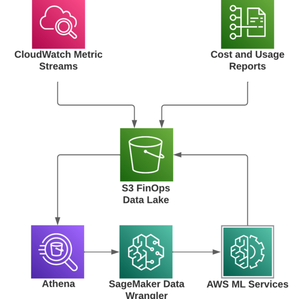
We recommend basing all forecasts on AWS SageMaker with the below architecture:

3.1. AWS Forecast

AWS Forecast is an easy-to-use AWS managed service which can be readily plugged into an AWS Step Function workflow triggered every week by a CloudWatch Event. The most suitable prediction algorithms to use are Prophet and DeepAR+ which are robust enough for identification of rapidly changing cycles / seasonality. Follow this article for set up steps.

3.2. AWS SageMaker AutoPilot

SageMaker hosts an engine for Jupyter notebooks. Autopilot is a library available in your code, to choose the right model for you. See this article.

3.3. AWS SageMaker Canvas

AWS SageMaker Canvas is the simplest service, introduced when SageMaker was released. The idea is a 100% drag and drop experience, fully automated, with zero decisions and code. See this article.

3.4. AWS SageMaker Serverless Inference

AWS SageMaker Serverless Inference doesn’t require a running instance, like Lambda functions. Instead, it’s provisioned and billed only when used. See the introductory articles for the AWS SageMaker Serverless Inference – this article and this article.

For cost and usage forecasting we recommend these algorithms:

1. Neural Prophet
2. N-BEATS
3. PyTorch Forecasting
4. AutoGluon

A special mention goes to Temporal Fusion Transformer, the current State of the Art.

Neural Prophet is one of the easiest to use and most robust algorithms. You need just four lines to produce a state-of-the-art forecast (the predicted values will be in the df_forecast dataframe):

from neuralprophet import NeuralProphet
import pandas as pd
df = pd.read_csv('./daily.csv')

model = NeuralProphet()
metrics = model.fit(df, freq="D")
df_forecast = model.make_future_dataframe(df, periods=365)
df_forecast = model.predict(df=df_forecast)

In addition to simplicity of use and robustness, Neural Prophet is one of the best documented forecasting library. See its discussion of cross-validation.

At the time of the writing of the article, the Neural Prophet does not include at the confidence interval over the predictions – Where to find yhat_lower and yhat_upper? · Discussion #270 · ourownstory/neural_prophet (github.com) which are critical – we recommend using the upper confidence interval of predicted values for budgetary purposes. You can use the branch mentioned in the GitHub post for yhat_upper.

4. Best Practices for Forecast Presentation

We recommend

• storing the forecast prediction values in an S3 data lake mergeable with the CloudWatch and CUR data lakes
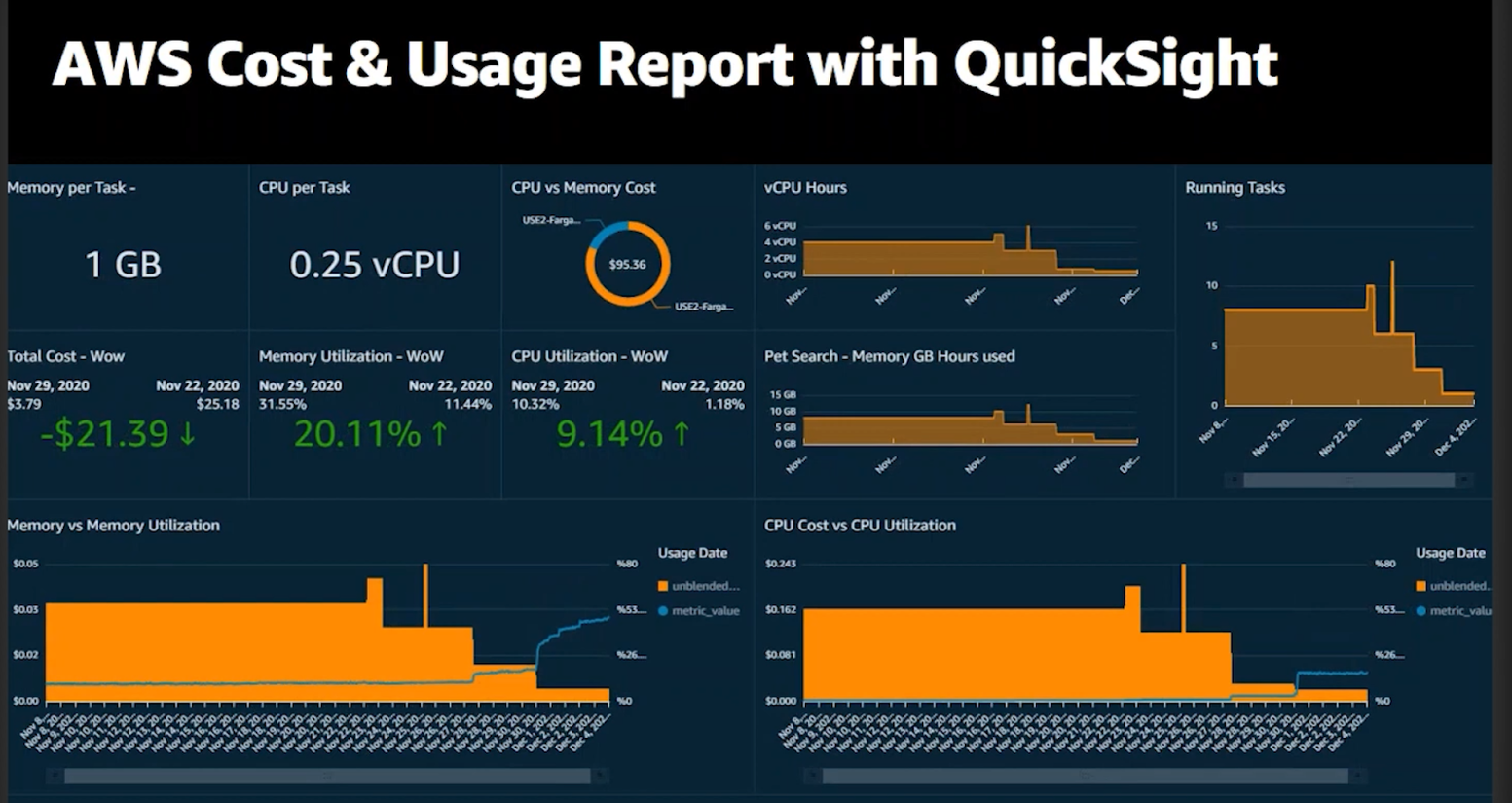
• visualizing the key metrics from the data lake in a number of AWS QuickSight dashboards, such as this one – see this article or this one or this one

5. Next Steps

We plan to deep dive into this topic in a future blog post, along with an worked out example with AWS SageMaker Serverless Inference. Please share your views on the ideal exact topic of the blog post.

6. References

• FinOs Foundation’s Best Practices for Forecasting

7. Publication Locations

This article is also published at Ermanno’s website.