
The Kronos foundation model — a transformer pretrained on 12.11 billion candlesticks from 96,569 assets across 45 exchanges — has collected 38,117 GitHub stars in fourteen months, an AAAI 2026 acceptance, and a fan base that believes it forecasts markets. A financial foundation model is a neural network pretrained once on decades of market history so it can forecast any instrument without task-specific training — the GPT playbook, pointed at OHLCV bars instead of text: feed Kronos 90 daily candles of AAPL and it emits the next 10, no fitting required.
Every one of those 38,117 stargazers faces the same unanswered question: how do you validate a model pretrained on the very history you would backtest it on?
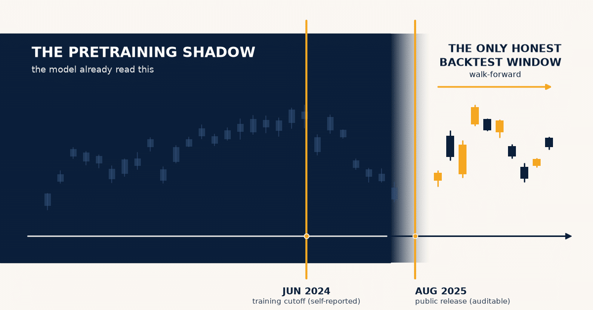
TL;DR: Kronos was pretrained on data through June 2024 and released in August 2025 (arXiv 2508.02739). Any backtest touching pre-release data measures recall, not foresight — I call this span the pretraining shadow. Community tests outside the shadow found the paper’s headline correlation of ~0.07 collapsing to +0.022 with a t-statistic of 1.39 — indistinguishable from zero and gone after transaction costs (issue #375). Below: the evidence, the Release-Date Rule, a runnable walk-forward protocol on QuantConnect/LEAN + AWS — the stack from my book — and four ways Kronos could still earn a place in production.
Why is everyone suddenly pretraining on candlesticks?
Three forces converged: the LLM playbook became a template (pretrain big, publish a leaderboard — Kronos applies it faithfully with a hierarchical tokenizer over OHLCV bars feeding an autoregressive transformer, Shi et al., 2025); GPU time got cheap enough that a 102M-parameter model trains on an academic budget; and — the incentive that matters — stars, citations, and acceptance letters pay out on benchmark tables, not on P&L. Nobody at AAAI asks for your slippage model.
That last force explains what the paper optimizes for and what it quietly omits. It reports Information Coefficient and excess return but not a single Sharpe ratio, and its flagship trading simulation — a 21.93% annualized excess return on China’s CSI 300 (paper, investment simulation) — comes from Kronos-large, the one model the team never released. Mini, small, and base are on Hugging Face; the 499M-parameter model behind the headline number is not. The best backtest belongs to the model you cannot run.
(Information Coefficient (IC) is the correlation between predicted and realized returns across stocks. Example: IC = 0.07 explains roughly half a percent of return variance — tiny per name, potentially tradable across hundreds of names, utterly hostage to costs.)
The contamination problem language models don’t have
When GPT-4 memorizes Wikipedia, it still generalizes — there are infinitely many new sentences to write. Markets differ in kind, not degree: there is exactly one realized price path. A language model’s test set can be freshly written; a market model’s test set is the training set’s future, and that future already happened by the time you run your backtest. This is the axis I mapped in the Anti-Alpha Paradox: for pretrained models, capability and contamination are one problem wearing two names.
I call the affected span the pretraining shadow: the stretch of market history a foundation model ingested before its weights froze. Every backtest inside the shadow measures memory. Kronos’s shadow covers everything through June 2024 — a beautiful 2019–2023 Kronos backtest is no more evidence of skill than my recalling yesterday’s closing prices makes me a forecaster.
You have seen this movie. In January, r/LocalLLaMA benchmarked nine LLMs on 25 stock-direction cases from 2024–2025 and crowned Claude Opus with 96% accuracy — before the author conceded the models “had already been trained on available public data” and the results were “unlikely to be replicated in real-time trading” (r/LocalLLaMA). Ninety-six percent accuracy is not a forecast. It is a bibliography.
Nor is it just hobbyists: on 18.1 million out-of-sample daily observations across 10,171 US securities, zero-shot TSFMs — Chronos, TimesFM — produce negative out-of-sample R² on returns, trailing plain gradient boosting (Re(Visiting) TSFMs in Finance). Quant researcher Jonathan Kinlay’s verdict on Kronos: the benchmarks are statistical, not economic — “economically exploitable returns after costs remains unproven” (Kinlay, 2026).
What the paper claims — and what post-shadow tests found
To the authors’ credit, the paper does hold out a temporal test window: pretraining stops June 2024, evaluation starts July 2024, reporting an IC near 0.07 and RankIC gains of +93% over the best competing foundation model. The problems start where the paper stops:
- The cutoff is unverifiable. The training corpus is not public; users asking for per-model cutoff details got no answer (issue #265).
- Fourteen months of silent selection. Between cutoff and release, the authors could watch candidate checkpoints perform on “held-out” 2024–25 data — and choose what to publish. Hedge funds know this trick as the incubation track record: launch ten funds, market the survivor.
- One window, one market, no deflation. The trading simulation is a single top-k backtest on Chinese A-shares at 0.15% cost per trade — no walk-forward, no adjustment for configurations tried.
Then the community ran the honest tests, strictly post-cutoff:
| Test | Setup | Result |
|---|---|---|
| Issue #354 | AAPL daily, 1,800 rolling forecasts, 2024-07 → 2026-07 | Underperforms a naive persistence baseline; directional accuracy 48.5–54.3% |
| Issue #355 | 30-min US bars, 8 symbols, walk-forward, frozen + fine-tuned | Fine-tuning improved token loss but not trading outcomes; worse than last-price naive in 3 of 4 periods |
| Issue #375 | Cross-sectional ranking, 182 US equities incl. 64 fallen names, 85 rebalances, 2024-07 → 2026-07, paper’s exact settings | IC = +0.022, Newey-West t = 1.39, positive in all four sub-periods, not significant, fails after transaction costs |
From 0.07 in the paper to 0.022 outside the shadow — a two-thirds haircut, landing below significance. The #375 author also quantified why point-in-time universes matter: his survivors-only universe returned a +143% median versus +7% for the honest list keeping the fallen names. Survivorship bias alone can manufacture a career.
The intent investigation. The stated reason quant Twitter is euphoric — “an open-source foundation model that predicts markets” (the hype is real) — does not survive the issues tab. The real reasons for 38,117 stars: the demo chart looks uncanny (it should — it is reconstructing patterns it ate), starring is free, and no stargazer has money at stake. The only party whose incentives align with truth is the one about to allocate capital — so the honest protocol has to come from practitioners.
The Release-Date Rule
The decision rule I now apply:
The Release-Date Rule: evaluate a pretrained market model only on data created after its public release date. Not the claimed training cutoff — the release date. If your backtest starts before the release date, you are not testing the model. You are testing its memory.
Why release date and not cutoff? Inversion — the mental model of asking how I would fake the result. If I wanted to ship a lookalike oracle, I would: (a) keep the training data private so no one can audit the cutoff, (b) evaluate on the year right after my cutoff while iterating checkpoints until that year looks good, and (c) release only the checkpoint that won. Each move is undetectable from outside — except through data the model provably could not have seen and the authors provably could not have selected on: data created after release. The Release-Date Rule is the only evaluation window that survives inversion.
History already ran this experiment. In 1999, Sullivan, Timmermann and White tested 7,846 technical trading rules on a century of Dow Jones data. In-sample, the best rules looked significant even after adjusting for data-snooping; in the honest out-of-sample decade, 1987–1996, the best rule’s edge reversed completely and lost significance (Sullivan, Timmermann & White, Journal of Finance 54(5)). We have since replaced 7,846 rules with 102 million parameters, and the null hypothesis has not moved an inch.
The vivid analogy is older still: past-posting — the wire con immortalized in The Sting, where the mark bets on a horse race that has already finished, because the bookmaker’s wire is delayed. A backtest inside the pretraining shadow is past-posting with extra steps: the model already knows how the race ended, and the backtest report is the delayed wire. The con works because the mark wants to believe the bet is live.
By accident of timing, the honest experiment is finally possible: Kronos now has thirteen months of guaranteed post-release data. Almost nobody has used it. Here is how to.
The honest protocol on QuantConnect, LEAN, and AWS
This is the validation stack from Hands-On AI Trading with Python, QuantConnect, and AWS (Wiley, 2025) — where we built a full strategy around Amazon’s Chronos foundation model and learned these guardrails the hard way. Three stages, with a firewall between them: score offline, trade from a static file, deflate the result. The model never runs inside the backtest — the offline-scoring guardrail from my Anti-Alpha experiments, where moving a single wall-clock date collapsed a Sharpe of 6.54 to 1.22.
Stage 1 — walk-forward scoring on AWS. A GPU spot instance walks Kronos-small through every rebalance date strictly after 2025-08-02, seeing only data available at that date:
RELEASE_DATE = "2025-08-02"   # arXiv v1; weights public
LOOKBACK, HORIZON = 90, 10    # the paper's own settings

tokenizer = KronosTokenizer.from_pretrained("NeoQuasar/Kronos-Tokenizer-base")
model = Kronos.from_pretrained("NeoQuasar/Kronos-small")
predictor = KronosPredictor(model, tokenizer, device="cuda:0", max_context=512)

def score_symbol(df, calendar, rebalance_dates):
    """Signal = mean of H predicted closes vs last close (paper's rule)."""
    signals = {}
    for t in rebalance_dates:
        assert t > pd.Timestamp(RELEASE_DATE), "inside the pretraining shadow"
        window = df.loc[:t].tail(LOOKBACK)          # data through t only
        pred = predictor.predict(
            df=window[["open", "high", "low", "close", "volume", "amount"]],
            x_timestamp=window.index.to_series(),
            y_timestamp=future_trading_days(calendar, t, HORIZON),
            pred_len=HORIZON,
            T=0.6, top_p=0.9, sample_count=10,      # paper's inference settings
        )
        signals[t] = pred["close"].mean() / window["close"].iloc[-1] - 1.0
    return pd.Series(signals)
Stage 2 — the LEAN backtest. QuantConnect’s engine trades the static signal file with Interactive Brokers fee and slippage models — the reality-modeling layer most README backtests skip:
class KronosReleaseDateRule(QCAlgorithm):
    TOP_K = 10

    def initialize(self):
        self.set_start_date(2025, 8, 4)      # first session AFTER release
        self.set_cash(1_000_000)
        self.set_brokerage_model(BrokerageName.INTERACTIVE_BROKERS_BROKERAGE,
                                 AccountType.MARGIN)
        raw = self.object_store.read("kronos/kronos_signals.csv")
        frame = pd.read_csv(io.StringIO(raw), index_col=0, parse_dates=True)
        self.signals = {d.date(): row.dropna().to_dict()
                        for d, row in frame.iterrows()}
        self.add_universe_selection(ManualUniverseSelectionModel(
            [Symbol.create(t, SecurityType.EQUITY, Market.USA)
             for t in frame.columns]))
        spy = self.add_equity("SPY", Resolution.DAILY).symbol
        self.schedule.on(self.date_rules.every_day(spy),
                         self.time_rules.after_market_open(spy, 30),
                         self.rebalance)

    def rebalance(self):
        scores = self.signals.get(self.time.date())
        if not scores:
            return
        ranked = sorted(scores, key=scores.get, reverse=True)[:self.TOP_K]
        for h in self.portfolio.values():
            if h.invested and h.symbol.value not in ranked:
                self.liquidate(h.symbol)
        for t in ranked:
            self.set_holdings(t, 1.0 / self.TOP_K)
Stage 3 — deflate for every config you tried. (The Deflated Sharpe Ratio (DSR) converts an observed Sharpe into the probability the true Sharpe exceeds zero, given how many configurations you tried and how ugly the returns are. Try 24 configs and report the best — the DSR asks whether it still impresses after admitting the other 23.) Implementing Bailey & López de Prado (2014):
EMC = 0.5772156649015329  # Euler–Mascheroni constant

def expected_max_sharpe(n_trials, sr_std):
    z = ((1 - EMC) * norm.ppf(1 - 1 / n_trials)
         + EMC * norm.ppf(1 - 1 / (n_trials * np.e)))
    return sr_std * z

def deflated_sharpe_ratio(sr_obs, n_trials, n_obs, skew, kurt, sr_std):
    """P[true SR > 0] after admitting every configuration you tried."""
    sr0 = expected_max_sharpe(n_trials, sr_std)
    num = (sr_obs - sr0) * np.sqrt(n_obs - 1)
    den = np.sqrt(1 - skew * sr_obs + (kurt - 1) / 4 * sr_obs ** 2)
    return norm.cdf(num / den)
Full listings for all three stages are in the post’s companion files; total footprint is under 200 lines.
What a README Sharpe looks like after the protocol
Run the arithmetic on a realistic scenario — a worked example, not a backtest claim. You test Kronos over the 13 post-release months (~264 trading days), try 24 configurations (two lookbacks × two horizons × two temperatures × three portfolio sizes — a modest search), and your best run shows an annualized Sharpe of 1.5 with mildly ugly returns (skew −0.5, kurtosis 5). The deflated Sharpe comes out at 0.71 — a 71% probability the true Sharpe exceeds zero, far below the conventional 95% bar. The sobering companion number: across 24 zero-skill configs on pure noise, the expected best Sharpe is 0.94. Your search procedure alone manufactures a Sharpe near one.
That is the base rates mental model doing its job: before believing any number, ask what the pipeline produces when there is nothing to find. And the second-order effect compounds it: 38,117 stargazers running variants of the same open-source signal are not independent experiments — whatever weak edge exists in a public model’s public signal is being arbitraged by its own popularity, the fate of every published anomaly since the momentum papers. The model proposes; the crowd disposes.
Four ways Kronos could actually earn its keep
The honest evidence does not say “worthless” — it says “not a zero-shot oracle.” Four uses survive the Release-Date Rule:
- Cross-sectional ranking feature, not forecaster. The post-shadow IC of +0.022 was insignificant but positive in all four sub-periods — the signature of a weak, possibly real ranking signal. As one feature inside a gradient-boosting stack, 2 bps of rank correlation can earn its slot. As a standalone strategy, it dies at the first commission.
- Volatility, not returns. Kronos’s realized-volatility forecasts hit R² ≈ 0.25 versus 0.23 for GARCH, with 9% lower MAE (paper). Volatility is persistent, so this is a low bar — but a real one, usable in position sizing, options overlays, and risk engines.
- Disciplined fine-tuning on post-cutoff data. The Re(Visiting) study found finance-pretrained models do add value when trained chronologically with expanding windows (arXiv 2511.18578). Fine-tune annually on data through year N, trade year N+1, never look back across the wall. Caveat: issue #355 found fine-tuning improved token loss but not trading outcomes — token-level objectives and P&L are different gods.
- Synthetic scenario generation. Kronos’s tokenizer-decoder is a generative model of plausible candlestick sequences. Sampling counterfactual paths to stress-test execution algos is a use case where memorizing history is a feature — you want realistic history-shaped paths, not alpha.
The decision rule for a head of quant
If your team wants Kronos (or any pretrained market model) in research, the checklist is five lines: (1) evaluate strictly post-release-date, no exceptions; (2) point-in-time universe with the dead names in it; (3) full cost and slippage modeling in LEAN or equivalent; (4) deflated Sharpe with an honest trial count, including deleted runs; (5) claims scoped to what was tested — a vol forecast is not an alpha, a ranking feature is not a strategy. Any pitch that opens with a chart from inside the pretraining shadow ends the meeting.
Alternative Perspectives
“The paper’s July-2024+ evaluation already is out-of-sample.” Partially fair — the authors did better than most. But an unverifiable cutoff plus fourteen months of possible checkpoint selection is exactly the gap the Release-Date Rule closes. Trust arrives with auditability, not assertion.
“IC 0.022 across thousands of stocks is a business.” With netting and near-zero costs, weak signals can compound — legitimate for a multi-strat desk with sub-basis-point execution, irrelevant for a stargazer with a retail account. Even then, t = 1.39 says you cannot yet reject luck.
“Everything is contaminated by this standard — human quants read history too.” True, and the difference is falsifiability: a human’s memory cannot be audited; a model’s release date can. That asymmetry argues for more foundation models with signed data manifests — see prediction one.
Three dated predictions
- By 31 December 2027, at least one major financial foundation model ships with a cryptographically signed training-data manifest (assets × dates), because allocators will refuse to diligence anything less.
- By mid-2027, a public leaderboard scoring TSFMs only on post-release windows exists and substantially reorders today’s benchmark tables.
- By end-2027, no peer-reviewed replication shows Kronos-class zero-shot models delivering significant after-cost US equity alpha in a strictly post-release window. I will publish a correction if one does.
Source Code
Stage 1: Offline walk-forward scoring
"""
Stage 1 of the Release-Date Rule protocol: offline walk-forward scoring.

Runs Kronos (github.com/shiyu-coder/Kronos) over a strictly post-release
window and writes one signal file that the LEAN backtest consumes.
Run this on an AWS GPU instance (g5.xlarge spot works) or AWS Batch —
the same research/backtest separation used throughout "Hands-On AI
Trading with Python, QuantConnect, and AWS" (Wiley, 2025).

Nothing in this file may read a bar dated after the rebalance date t.
"""

import pandas as pd

# From the Kronos repo (pip install -r requirements.txt, then repo root)
from model import Kronos, KronosTokenizer, KronosPredictor

RELEASE_DATE = "2025-08-02"   # arXiv v1 of the Kronos paper; weights public
LOOKBACK = 90                 # paper's investment-simulation lookback
HORIZON = 10                  # paper's forecast horizon H (trading days)

tokenizer = KronosTokenizer.from_pretrained("NeoQuasar/Kronos-Tokenizer-base")
model = Kronos.from_pretrained("NeoQuasar/Kronos-small")
predictor = KronosPredictor(model, tokenizer, device="cuda:0", max_context=512)


def future_trading_days(calendar: pd.DatetimeIndex, t: pd.Timestamp, n: int) -> pd.Series:
    """Next n exchange sessions strictly after t, from a point-in-time calendar."""
    return pd.Series(calendar[calendar > t][:n])


def score_symbol(df: pd.DataFrame, calendar: pd.DatetimeIndex,
                 rebalance_dates: list[pd.Timestamp]) -> pd.Series:
    """
    Signal = (mean of H predicted closes) / last close - 1
    — the exact signal definition from the Kronos paper's investment
    simulation, applied only on dates after RELEASE_DATE.
    """
    signals = {}
    for t in rebalance_dates:
        assert t > pd.Timestamp(RELEASE_DATE), "inside the pretraining shadow"
        window = df.loc[:t].tail(LOOKBACK)          # data through t only
        if len(window) < LOOKBACK:
            continue
        pred = predictor.predict(
            df=window[["open", "high", "low", "close", "volume", "amount"]],
            x_timestamp=window.index.to_series(),
            y_timestamp=future_trading_days(calendar, t, HORIZON),
            pred_len=HORIZON,
            T=0.6, top_p=0.9, sample_count=10,      # paper's inference settings
        )
        signals[t] = pred["close"].mean() / window["close"].iloc[-1] - 1.0
    return pd.Series(signals, name="kronos_signal")


if __name__ == "__main__":
    # universe.parquet: point-in-time constituents to avoid survivorship bias.
    # Fallen names must stay in the file — see GitHub issue #375, where the
    # survivors-only version of the same universe returned +143% median
    # versus +7% for the full point-in-time list.
    universe = pd.read_parquet("universe.parquet")
    calendar = pd.DatetimeIndex(pd.read_parquet("calendar.parquet")["date"])
    rebalances = [d for d in calendar if d > pd.Timestamp(RELEASE_DATE)][::5]

    rows = []
    for ticker, df in universe.groupby("ticker"):
        s = score_symbol(df.set_index("date").sort_index(), calendar, rebalances)
        rows.append(s.rename(ticker))
    signals = pd.concat(rows, axis=1)
    signals.to_csv("kronos_signals.csv")           # -> LEAN ObjectStore
    print(f"{signals.shape[1]} symbols x {signals.shape[0]} rebalance dates")
Stage 2 – the Lean Backtest
"""
Stage 2 of the Release-Date Rule protocol: the LEAN backtest.

A QuantConnect algorithm that consumes the pre-computed Kronos signals
(Stage 1) from the ObjectStore and trades a cost-loaded top-k portfolio
strictly after the model's public release date. The model runs offline;
the backtest only reads a static signal file — the same offline-scoring
guardrail I used in the Anti-Alpha Paradox experiments.

Backtest window: 2025-08-04 (first session after release) onward.
"""

from AlgorithmImports import *
import io
import pandas as pd


class KronosReleaseDateRule(QCAlgorithm):

    TOP_K = 10

    def initialize(self):
        self.set_start_date(2025, 8, 4)      # first session AFTER release
        self.set_end_date(2026, 8, 28)
        self.set_cash(1_000_000)

        # Reality modeling: fees, spread-crossing slippage, no free fills.
        self.set_brokerage_model(BrokerageName.INTERACTIVE_BROKERS_BROKERAGE,
                                 AccountType.MARGIN)
        self.universe_settings.resolution = Resolution.DAILY

        raw = self.object_store.read("kronos/kronos_signals.csv")
        frame = pd.read_csv(io.StringIO(raw), index_col=0, parse_dates=True)
        self.signals = {d.date(): row.dropna().to_dict()
                        for d, row in frame.iterrows()}

        tickers = frame.columns.tolist()
        symbols = [Symbol.create(t, SecurityType.EQUITY, Market.USA)
                   for t in tickers]
        self.add_universe_selection(ManualUniverseSelectionModel(symbols))

        self.spy = self.add_equity("SPY", Resolution.DAILY).symbol
        self.schedule.on(self.date_rules.every_day(self.spy),
                         self.time_rules.after_market_open(self.spy, 30),
                         self.rebalance)

    def rebalance(self):
        scores = self.signals.get(self.time.date())
        if not scores:
            return                            # not a rebalance date
        ranked = sorted(scores, key=scores.get, reverse=True)[:self.TOP_K]
        targets = {t: 1.0 / self.TOP_K for t in ranked}

        for holding in self.portfolio.values():
            if holding.invested and holding.symbol.value not in targets:
                self.liquidate(holding.symbol)
        for ticker, weight in targets.items():
            self.set_holdings(ticker, weight)

    def on_end_of_algorithm(self):
        self.log(f"Final equity: {self.portfolio.total_portfolio_value:,.0f}")
        # Export daily equity for Stage 3 (deflated Sharpe) via ObjectStore.
Stage 3 – Deflate the Sharpe Ratio
"""
Stage 3 of the Release-Date Rule protocol: deflate the Sharpe ratio.

Implements the Deflated Sharpe Ratio of Bailey & Lopez de Prado (2014),
"The Deflated Sharpe Ratio: Correcting for Selection Bias, Backtest
Overfitting and Non-Normality", Journal of Portfolio Management 40(5).

Every config you tried — every lookback, horizon, temperature, top-k —
raises the bar your final Sharpe must clear. Count them all, including
the runs you deleted.
"""

import numpy as np
from scipy.stats import norm

EMC = 0.5772156649015329  # Euler-Mascheroni constant


def expected_max_sharpe(n_trials: int, sr_std: float) -> float:
    """E[max SR] across n_trials of zero-skill strategies (daily units)."""
    z = ((1 - EMC) * norm.ppf(1 - 1 / n_trials)
         + EMC * norm.ppf(1 - 1 / (n_trials * np.e)))
    return sr_std * z


def deflated_sharpe_ratio(sr_obs: float, n_trials: int, n_obs: int,
                          skew: float, kurt: float, sr_std: float) -> float:
    """
    P[true SR > 0], given the observed daily SR, the number of configs
    tried, the sample length, and the non-normality of returns.
    """
    sr0 = expected_max_sharpe(n_trials, sr_std)
    num = (sr_obs - sr0) * np.sqrt(n_obs - 1)
    den = np.sqrt(1 - skew * sr_obs + (kurt - 1) / 4 * sr_obs ** 2)
    return norm.cdf(num / den)


if __name__ == "__main__":
    # Worked example from the post: a README-grade annualized Sharpe of 1.5
    # over ~12.5 months of daily data (264 obs), after trying 24 configs,
    # with mildly ugly returns (skew -0.5, kurtosis 5) and a cross-trial
    # daily-SR dispersion of 0.03.
    daily_sr = 1.5 / np.sqrt(252)
    dsr = deflated_sharpe_ratio(daily_sr, n_trials=24, n_obs=264,
                                skew=-0.5, kurt=5.0, sr_std=0.03)
    noise = expected_max_sharpe(24, 0.03) * np.sqrt(252)
    print(f"Deflated Sharpe (confidence true SR > 0): {dsr:.2f}")   # ~0.71
    print(f"Best Sharpe 24 zero-skill configs 'find': {noise:.2f}")  # ~0.94
FAQ
What is the Kronos foundation model?
An open-source transformer from Tsinghua University pretrained on 12.11 billion K-line records from 96,569 assets across 45 exchanges. It tokenizes OHLCV bars and forecasts future bars zero-shot. Three sizes are public (4.1M–102.3M parameters); the 499M flagship is not (GitHub).
Can I trade profitably with Kronos out of the box?
The strictly post-cutoff evidence says no: near coin-flip directional accuracy on single names (#354) and a cross-sectional IC of +0.022 that is insignificant and disappears after costs (#375).
How do I validate a time series foundation model honestly?
Apply the Release-Date Rule: evaluate only on data created after public release, walk forward, use a point-in-time universe, load full transaction costs, and deflate the Sharpe for every configuration tried. The three-stage protocol above implements this end to end.
Is Kronos better than Chronos or TimesFM for finance?
On the paper’s benchmarks, yes — RankIC +93% over the best general-purpose TSFM. But independent work finds zero-shot TSFMs as a class produce negative out-of-sample R² on equity returns (Re(Visiting)). Beating Chronos at a game Chronos loses is not a trading edge. For the constructive path — including the Chronos strategy we built on QuantConnect and AWS — see my book.
Disclaimer: This reflects my personal views and experience, not financial advice. Past performance doesn’t guarantee future results.
Jiri Pik is the founder and CEO of RocketEdge.com, where he builds AI trading systems and cloud-native architecture for financial firms. He is a co-author of Hands-On AI Trading with Python, QuantConnect, and AWS (Wiley, 2025). He writes at jiripik.com about AI, quantitative finance, and systems thinking — usually 6–18 months before it hits mainstream.