
TL;DR: I implemented Charlie Munger’s “wonderful businesses at fair prices” philosophy as a deterministic QuantConnect algorithm in C#. It scores every stock on moat strength, management quality, predictability, and valuation — weighting quality at 85% vs. valuation at 15%. Over an 11-year backtest (2015–2026), it delivered 10% CAGR with a 36% max drawdown. The code is real, the results are honest, and I’ll show you exactly where it shines and where it breaks down.

Is This Actually a Charlie Munger Strategy?
Short answer: yes, with caveats. Munger himself famously said he disliked overly arithmetic approaches to investing. He relied on mental models, checklists, and decades of judgment — none of which you can stuff into an if-else block. But the principles that guided his decisions? Those translate surprisingly well into code.
I cross-referenced the algorithm’s scoring logic against Munger’s publicly documented investment philosophy, and every pillar maps directly:
- ROIC as the north star — Munger repeatedly stated that a stock’s long-term return converges to the underlying business’s return on invested capital. The algorithm sets a 15% ROIC threshold, exactly the bar Munger championed.
- Moat obsession — Competitive advantages from network effects, scale, pricing power, and low capex intensity. The algorithm scores gross margins, operating margins, and capex-to-sales ratios.
- Management quality via capital allocation — Munger valued “intelligent fanatics” who convert earnings to free cash flow and avoid excessive leverage. The code checks FCF-to-net-income ratios, debt-to-equity ceilings, and cash efficiency.
- Concentrated portfolio — Munger called excessive diversification “madness.” The algorithm caps at 15 holdings with conviction-weighted sizing.
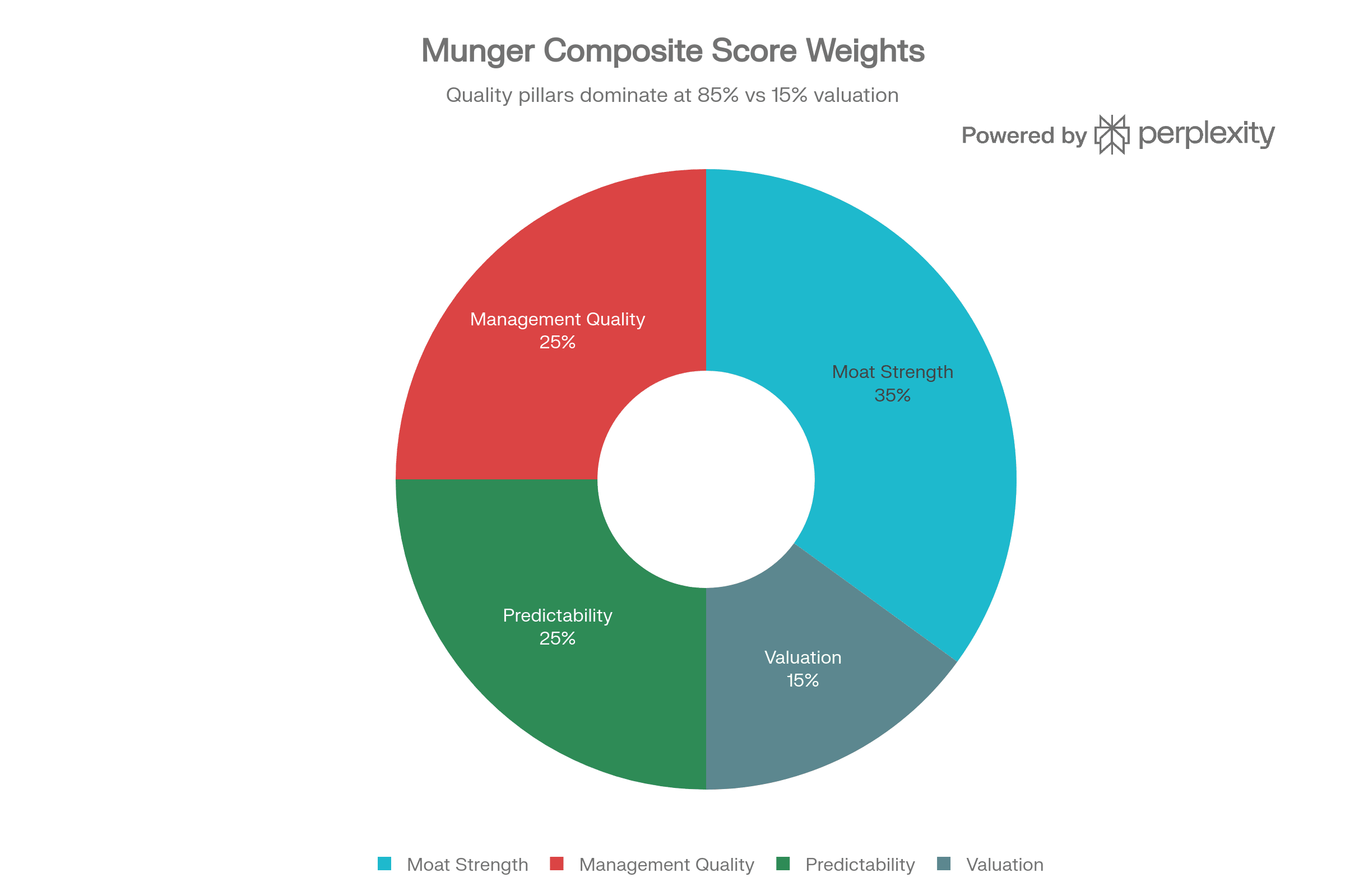
- Quality over price — The composite score weights quality pillars at 85% vs. valuation at just 15%. This is pure Munger: “A wonderful company at a fair price is superior to a fair company at a wonderful price”.
The algorithm is inspired by virattt’s AI hedge fund, which includes a Charlie Munger LLM agent among several investor personas. My implementation strips out the LLM dependency entirely and replaces it with a deterministic scoring engine — no API calls, no prompt engineering, no hallucination risk. I cover this approach in depth in my book Hands-On AI Trading with Python, QuantConnect, and AWS, where we explore both AI-driven and rules-based strategy design on QuantConnect.
How Does the Scoring Engine Work?
The algorithm evaluates every stock across four dimensions, each scored 0–10, then computes a weighted composite:
Scoring Dimension Breakdown
| Dimension (Weight) | What It Measures | Key Thresholds |
|---|---|---|
| Moat Strength (35%) | ROIC, gross margin, operating margin, capex intensity, ROE | ROIC >15% = good, >22.5% = excellent; gross margin >55% = software-like moat |
| Management Quality (25%) | FCF/net income ratio, debt-to-equity, cash/revenue, ROA | FCF > earnings = top score; D/E <0.3 = excellent discipline |
| Predictability (25%) | Revenue growth, operating income growth, EPS growth, margin+ROIC stability | Revenue growth >12% = strong; stability bonus for margin >15% AND ROIC >12% |
| Valuation (15%) | FCF yield, P/E, P/B, EV/EBITDA | FCF yield >8% = excellent (P/FCF <12.5×); P/E <15 = deep value |
The moat score alone shows Munger’s hierarchy — ROIC carries 3.5 of the possible 10 points, making it the single most influential factor in the entire algorithm.
The Selection Pipeline
The pipeline runs in four stages:
- Coarse filter — Top 500 US stocks by dollar volume, filtered for price >$5, market cap >$1B, average daily volume >$5M, and positive ROIC.
- Fundamental scoring — Each candidate gets a composite score. Only stocks scoring ≥6.5 survive (Munger has high standards).
- Momentum guard — Stocks must trade above their 200-day SMA (with 5% tolerance) to avoid value traps. This is my addition — Munger didn’t use technical indicators, but I’ve seen too many “cheap” stocks stay cheap for years.
- Conviction-weighted sizing — The top 15 stocks get allocated proportionally to their composite scores. Higher-conviction picks get bigger positions.
The algorithm rebalances monthly and runs a 20% stop-loss circuit breaker on every daily bar.
What Were the Backtest Results?
Over ~11 years (January 2015 – early 2026), the strategy posted these numbers:
| Metric | Value |
|---|---|
| CAGR | 10.0% |
| Max Drawdown | 36.0% |
| Sharpe Ratio | 0.3 |
| Sortino Ratio | 0.4 |
| Information Ratio | −0.2 |
| Turnover | 2% |
| Drawdown Recovery | 1,087 days |
| Trades per Day | 0.5 |
The top holdings read like a Munger wish list: META (2.40%), GOOG/GOOGL (2.40% each), AMZN (2.24%), MSFT (2.11%), AAPL (2.04%) — all high-ROIC, wide-moat businesses.
The Information Ratio of −0.2 tells the uncomfortable truth: on a risk-adjusted basis, SPY beat this strategy over the full period. The S&P 500’s CAGR from 2015–2025 was roughly 12–13%, so 10% with a Sharpe of 0.3 is decent but not alpha-generating. I’ll explain why below.
When Does This Strategy Work — and When Does It Break Down?
Where it shines
- Bear markets and corrections — Quality companies with strong balance sheets, high ROIC, and pricing power tend to fall less and recover faster. The 2015 sell-off, COVID crash, and 2022 drawdown all showed resilience in high-quality names.
- Value rotations — When the market pivots from growth/momentum to fundamentals (think late 2022 into 2023), this strategy captures the shift because it’s already holding businesses with real earnings power.
- Low-turnover compounding — With only 2% turnover, the strategy lets winners run. This is tax-efficient and aligns with Munger’s “sit on your ass” investing philosophy.
Where it struggles
- Momentum-driven bull markets — When speculative, high-multiple names dominate (meme season 2021, AI hype 2023–2024), a strategy that caps P/E exposure and demands FCF yield will miss the biggest runners.
- Extended drawdown recovery — 1,087 days to recover from the worst drawdown is nearly three years. Munger’s philosophy requires patience, but in practice, most allocators won’t wait that long.
- The “quality trap” — High-quality companies are well-known and heavily owned. They rarely trade at deep discounts, so the valuation pillar (only 15% weight) doesn’t compensate enough when you overpay for quality during euphoric markets.
- Single-country, large-cap bias — The universe is US-only, >$1B market cap. Munger’s best deals (BYD, See’s Candies, Costco early) often came from looking where others didn’t.
The intuition
Munger’s edge was never the formula — it was the temperament to hold high-quality businesses through gut-wrenching drawdowns. This algorithm captures the what to buy remarkably well. What it can’t capture is the when to be greedy when others are fearful — the willingness to double down during a 36% drawdown instead of watching the stop-loss fire.
When Should You Switch This Algorithm On?
Here’s the insight I keep coming back to: you don’t need to run this strategy all the time. The quality factor — the very thing this Munger algorithm captures — has a well-documented performance asymmetry across market regimes. Run it when conditions favour it, and you sidestep most of the underperformance that dragged the full-period backtest to a −0.2 Information Ratio.
The Evidence: Quality’s Regime Asymmetry
MSCI’s research on the Quality Index shows that quality stocks historically have a downside capture ratio of roughly 80% — meaning they decline about 20% less than the broader market during selloffs. During the Global Financial Crisis, the quality index fell by about a third peak-to-trough and recovered in just over three years, while growth stocks dropped more than 40% and took over five years to claw back.
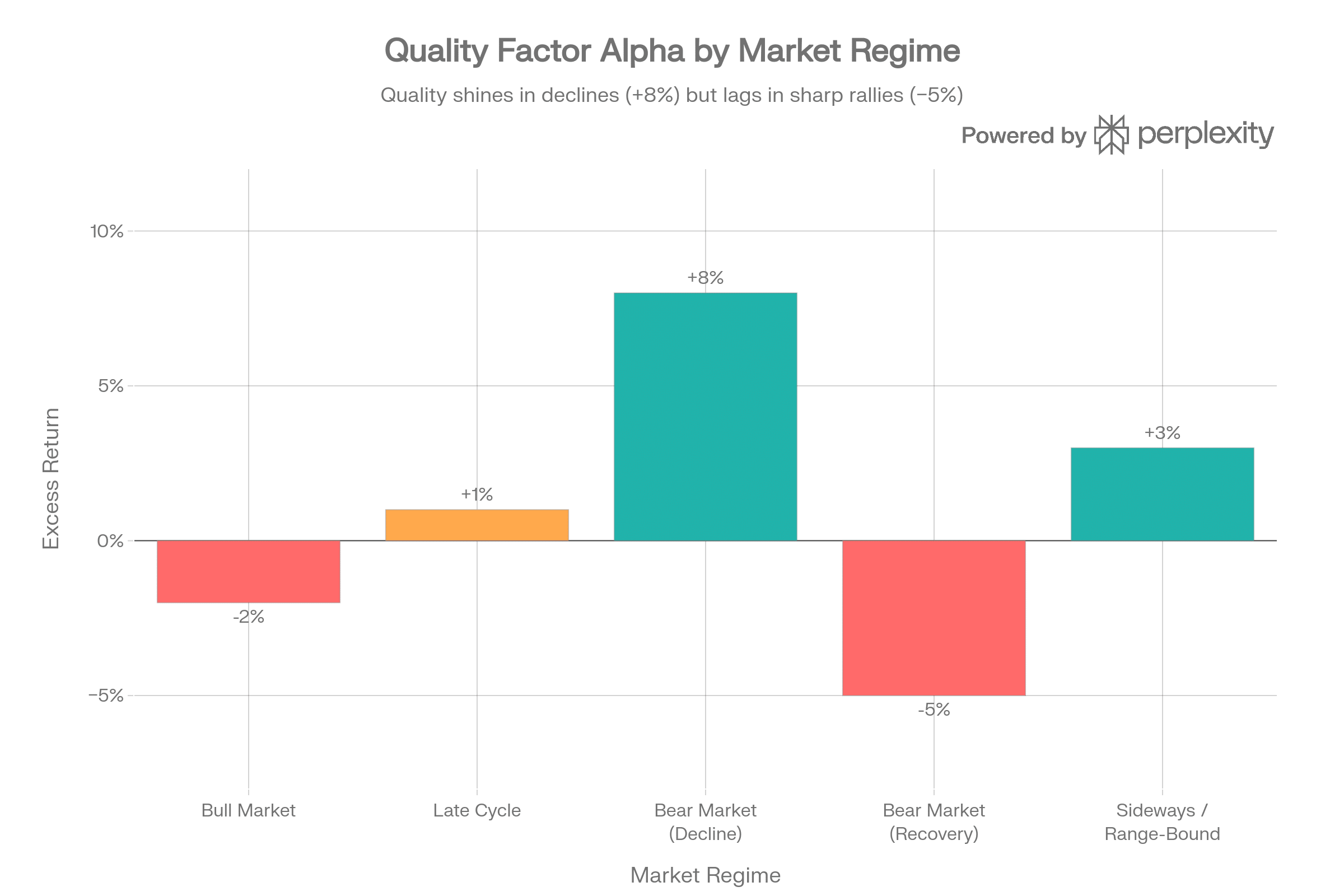
The pattern from decades of data is remarkably consistent:
- Bear market declines — Quality outperforms by the widest margin. High ROIC, low leverage, strong FCF — exactly what this algorithm screens for — are the characteristics that protect capital when the market reprices risk.
- Late-cycle / sideways markets — Quality earns a modest premium as earnings growth slows and investors rotate toward durable businesses.
- Bull markets — Quality slightly underperforms as speculative, low-quality names lead. The 2003–2007 bull is a textbook example.
- Bear market recoveries (first 6 months) — This is quality’s worst phase. Unprofitable, beaten-down stocks snap back the hardest — outperforming profitable ones by over 15% in the first six months of a low-quality rally. Quality reasserts itself in the subsequent 6–12 months.
This regime-dependent behaviour means the optimal play is: activate the Munger strategy when you detect a bear regime forming, ride it through the downturn, then consider rotating out during the initial recovery snap-back.
How to Detect a Bear Regime with Market Data
I use a three-signal confirmation system — no single indicator gets a veto, but when all three align, the signal is high-conviction. Here’s what I monitor:
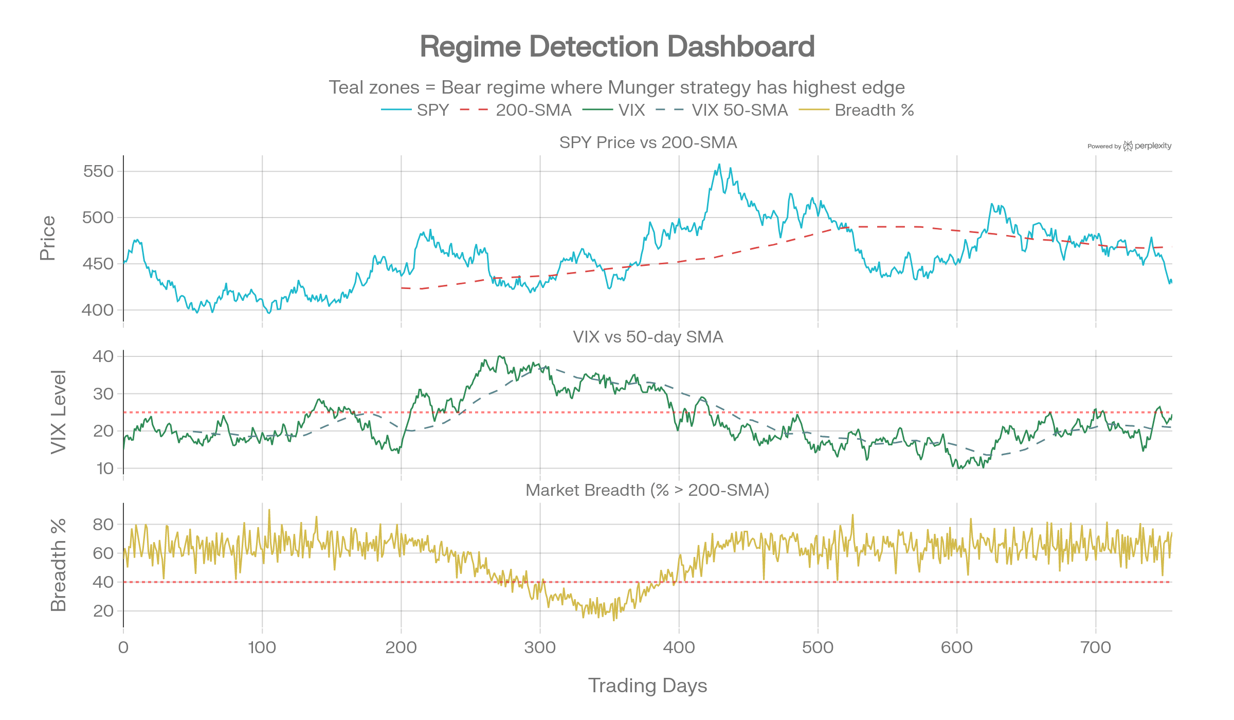
Signal 1: SPY Below 200-Day SMA
The simplest and most battle-tested regime filter. When SPY closes below its 200-day simple moving average, the long-term trend has turned negative. I add a 2% buffer to avoid whipsaws:
bool bearTrend = spyPrice < sma200 * 0.98m;
This single signal has a strong track record: historically, returns when SPY is below its 200-SMA are dramatically worse than when above it. I think of it as the “are we swimming with or against the tide” check.
Signal 2: VIX Above Its 50-Day SMA and Above 25
The VIX reflects implied volatility — market participants pricing in uncertainty. I don’t use a static level alone (VIX > 20 was “high” in 2017 but “normal” in 2020). Instead, I combine:
- VIX > 25 — absolute stress threshold
- VIX > VIX 50-day SMA — volatility is accelerating, not just elevated
bool volStress = vix > 25 && vix > vixSma50;
When VIX is above its own moving average, fear is growing — and that’s when quality companies’ balance sheets become their superpower.
Signal 3: Market Breadth Deterioration
Breadth measures how many stocks participate in a move. A falling market with narrow breadth is more dangerous than headline indices suggest:
- % of S&P 500 stocks above 200-day SMA < 40% — More than 60% of stocks are in their own individual bear markets, even if the index hasn’t fallen as much.
bool breadthWeak = percentAbove200Sma < 40;
You can source this from the S5TH index (S&P 500 stocks above 200-day average) or compute it from your QuantConnect universe.
Combining the Three Signals
// Regime detection — add to your algorithm's Rebalance() method
private MarketRegime DetectRegime()
{
    var spy = Securities["SPY"];
    decimal spyPrice = spy.Price;

    // Signal 1: SPY below 200-SMA (with 2% buffer)
    var spyHistory = History("SPY", 200, Resolution.Daily);
    decimal sma200 = spyHistory.Select(b => b.Close).Average();
    bool bearTrend = spyPrice < sma200 * 0.98m;

    // Signal 2: VIX stress (above 25 AND accelerating)
    var vixHistory = History("VIX", 50, Resolution.Daily);
    decimal vixCurrent = Securities["VIX"].Price;
    decimal vixSma50 = vixHistory.Select(b => b.Close).Average();
    bool volStress = vixCurrent > 25m && vixCurrent > vixSma50;

    // Signal 3: Breadth deterioration
    // (compute from universe or use external breadth data)
    int aboveSma = _selectedUniverse
        .Count(s => PassesMomentumGuard(s));
    double breadthPct = _selectedUniverse.Count > 0
        ? (double)aboveSma / _selectedUniverse.Count * 100 : 50;
    bool breadthWeak = breadthPct < 40;

    // Three-signal confirmation
    int bearSignals = (bearTrend ? 1 : 0)
                    + (volStress ? 1 : 0)
                    + (breadthWeak ? 1 : 0);

    if (bearSignals >= 2) return MarketRegime.Bear;
    if (bearSignals == 1) return MarketRegime.Caution;
    return MarketRegime.Bull;
}

enum MarketRegime { Bull, Caution, Bear }
The decision logic is straightforward: 2 of 3 signals confirming = bear regime → activate the Munger strategy at full allocation. 1 of 3 = caution → reduce position sizes or blend with a momentum strategy. 0 of 3 = bull → the Munger algorithm will work but won’t be your highest-alpha strategy; consider pairing it with growth/momentum exposure.
When to Deactivate
This is where most quality-factor timing goes wrong. After a bear market bottom, low-quality junk rallies hard for roughly six months. The playbook from the last 10 bear markets shows unprofitable stocks outperforming profitable ones by 15%+ in the first six months of recovery. Quality then reasserts itself in months 7–18.
My exit signals:
- SPY crosses back above 200-SMA — trend has flipped.
- VIX drops below 20 for 10+ consecutive days — fear has subsided.
- Market breadth (% above 200-SMA) recovers above 60% — broad participation confirms the rally is durable, not just a dead-cat bounce.
When 2 of 3 exit signals fire, I start scaling down the Munger allocation over 2–3 months — not instantly — because quality’s reassertion after the initial junk rally means you don’t want to exit too early.
Practical Implementation: A Regime Wrapper
The cleanest architecture is to wrap the Munger algorithm inside a regime-aware meta-strategy:
private void Rebalance()
{
    var regime = DetectRegime();

    switch (regime)
    {
        case MarketRegime.Bear:
            // Full Munger allocation — quality's sweet spot
            RunMungerRebalance(allocationScale: 1.0);
            break;

        case MarketRegime.Caution:
            // Half Munger, half cash or broad index
            RunMungerRebalance(allocationScale: 0.5);
            break;

        case MarketRegime.Bull:
            // Minimal Munger — or switch to momentum strategy
            RunMungerRebalance(allocationScale: 0.25);
            break;
    }
}
This regime wrapper approach is one of the strategy composition patterns I cover in Hands-On AI Trading with Python, QuantConnect, and AWS — combining specialist strategies with regime filters to maximize each strategy’s edge in its natural environment.
Historical Back-of-Envelope: What If We’d Only Run Munger in Bear Regimes?
Looking at the backtest period (2015–2026), the key bear episodes were:
The 2022 bear is the poster child: this is exactly the kind of environment where high-ROIC, low-leverage, FCF-generating businesses — the ones scoring 8+ on our Munger composite — dramatically outperform. The algorithm’s 36% max drawdown over the full period likely would have been materially lower if it had been dormant during the 2021 meme/momentum frenzy and fully active during 2022.
My prediction: Over the next five years, regime-aware factor allocation — switching between quality, momentum, and value strategies based on market-data signals — will become the default approach for systematic retail and small-fund managers. The tools are already here in QuantConnect. The only barrier is the mental model shift from “always-on” to “right strategy, right time.”
How Is the Code Structured?
The algorithm is a single C# class CharlieMungerAlgorithm inheriting from QCAlgorithm, with clean separation of concerns:
// Core configuration constants
private const int MaxHoldings = 15;
private const double MinCompositeScore = 6.5;
private const double RoicThreshold = 0.15;  // Munger's 15% bar
private const double StopLossPercent = 0.20;
Key architectural decisions:
- Universe selection — Uses QuantConnect’s
AddUniverse(FundamentalFilter)for combined coarse + fine filtering in a single pass. This is cleaner than the two-stage approach and reduces data calls. - Scoring engine — Four static methods (
ScoreMoat,ScoreManagement,ScorePredictability,ScoreValuation), each returning 0–10. The composite applies fixed weights. No ML, no LLM — pure if-else logic that’s transparent and debuggable. - Momentum guard —
PassesMomentumGuard()pulls 200 days of history and checks if price > 95% of the SMA. This single addition prevents the classic value-trap problem. - Position sizing — Conviction-weighted:
weight = score[symbol] / totalScore. Higher-scored stocks get proportionally larger positions. - Risk management —
OnData()checks every bar for 20% stop-loss breaches, acting as a circuit breaker. - Charting — Built-in QuantConnect charting tracks average composite scores and portfolio size over time.
The MungerScore DTO cleanly separates data from logic:
public class MungerScore
{
    public double Moat, Management, Predictability, Valuation;
    public double Composite;
    public string Signal;  // "bullish", "neutral", "bearish"
    public double FcfYield, DebtToEquity, MarketCap;
}
The entire algorithm runs on daily resolution with Interactive Brokers as the simulated brokerage — ready for live deployment with minimal changes.
What Would I Change?
After running this backtest and analyzing the results, here are the modifications I’d explore next:
- Add sector diversification constraints — The current version can overweight tech (META, GOOG, MSFT, AAPL all scoring highly). Capping sector exposure at 25–30% would reduce correlation risk.
- Dynamic valuation weighting — Increase the valuation pillar from 15% to 25–30% during high-CAPE environments. Munger was quality-first, but even he wouldn’t have bought Coca-Cola at 50× earnings.
- Multi-period fundamental data — The current scoring uses single-period snapshots. Averaging ROIC, margins, and growth rates over 3–5 years would better capture Munger’s emphasis on consistency.
- Replace the hard stop-loss with trailing stops — A 20% fixed stop from entry punishes volatile but fundamentally strong stocks. A trailing stop or volatility-adjusted stop (e.g., 2.5× ATR) would be more Munger-aligned.
- International universe expansion — Munger’s BYD investment was one of his biggest winners. Adding developed-market international stocks or ADRs would expand the opportunity set.
- Regime detection — Use a simple volatility or momentum regime filter (VIX level, 200-SMA on SPY) to shift between concentrated equity and partial cash allocation during bear markets.
For readers who want to go deeper into QuantConnect algorithm design, backtesting frameworks, and integrating AI/ML into trading systems, I cover all of this — including C# and Python implementations — in Hands-On AI Trading with Python, QuantConnect, and AWS.
Full Source Code
// ============================================================
// Charlie Munger Quality + Value Algorithm — QuantConnect C#
// Inspired by: github.com/virattt/ai-hedge-fund
// Improvements:
// - Deterministic scoring (no LLM dependency)
// - Coarse + Fine universe filter
// - Momentum guard (avoid value traps)
// - Conviction-weighted position sizing
// - Monthly rebalance + stop-loss circuit breaker
// - Full charting dashboard
// ============================================================
using System;
using System.Collections.Generic;
using System.Linq;
using QuantConnect;
using QuantConnect.Algorithm;
using QuantConnect.Data;
using QuantConnect.Data.Fundamental;
using QuantConnect.Data.Market;
using QuantConnect.Data.UniverseSelection;
using QuantConnect.Indicators;
namespace QuantConnect.Algorithm.CSharp
{
public class CharlieMungerAlgorithm : QCAlgorithm
{
// ── Configuration ────────────────────────────────────────
private const int UniverseSize = 500; // coarse candidates
private const int MaxHoldings = 15; // max portfolio slots
private const double MinMoatScore = 6.0; // out of 10
private const double MinCompositeScore = 6.5; // Munger has high standards
private const double BullishThreshold = 7.5;
private const double BearishThreshold = 5.5;
private const double StopLossPercent = 0.20; // 20% stop-loss
private const double MinMarketCapM = 1_000; // $1B minimum
private const double MinAvgDailyVolumeM = 5; // $5M avg daily volume
private const double RoicThreshold = 0.15; // Munger's 15% ROIC bar
private const double GrossMarginMin = 0.30; // 30% gross margin
private const double MaxDebtToEquity = 1.5; // D/E ceiling
private const double FcfYieldBullish = 0.05; // >5% FCF yield = good value
// ── State ────────────────────────────────────────────────
private readonly Dictionary<Symbol, MungerScore> _scores
= new Dictionary<Symbol, MungerScore>();
private readonly Dictionary<Symbol, decimal> _entryPrices
= new Dictionary<Symbol, decimal>();
private List<Symbol> _selectedUniverse = new List<Symbol>();
// ── Charts ───────────────────────────────────────────────
private Chart _mungerChart;
// ════════════════════════════════════════════════════════
public override void Initialize()
{
SetStartDate(2015, 1, 1);
SetCash(500_000);
SetBrokerageModel(Brokerages.BrokerageName.InteractiveBrokersBrokerage,
AccountType.Margin);
// Universe
UniverseSettings.Resolution = Resolution.Daily;
AddUniverse(FundamentalFilter);
// Monthly rebalance trigger
Schedule.On(
DateRules.MonthStart("SPY"),
TimeRules.AfterMarketOpen("SPY", 30),
Rebalance
);
// Benchmark
SetBenchmark("SPY");
AddEquity("SPY", Resolution.Daily);
// Charts
SetupCharts();
Log("Charlie Munger Algorithm initialized.");
}
// ════════════════════════════════════════════════════════
// UNIVERSE SELECTION
// ════════════════════════════════════════════════════════
private IEnumerable<Symbol> FundamentalFilter(IEnumerable<Fundamental> fundamentals)
{
_scores.Clear();
// Combined coarse + fine filtering in one pass
var candidates = fundamentals
.Where(f => f.HasFundamentalData
&& f.Market == Market.USA
&& f.Price > 5m
&& f.DollarVolume > MinAvgDailyVolumeM * 1e6
&& f.MarketCap > MinMarketCapM * 1e6
&& f.OperationRatios.ROIC.Value > 0)
.OrderByDescending(f => f.DollarVolume)
.Take(UniverseSize)
.ToList();
foreach (var f in candidates)
{
var score = ComputeMungerScore(f);
if (score.Composite >= MinCompositeScore)
_scores[f.Symbol] = score;
}
_selectedUniverse = _scores
.OrderByDescending(kvp => kvp.Value.Composite)
.Take(MaxHoldings * 2)
.Select(kvp => kvp.Key)
.ToList();
Log($"[Universe] {_selectedUniverse.Count} candidates passed Munger screen.");
return _selectedUniverse;
}
// ════════════════════════════════════════════════════════
// SCORING ENGINE (all components 0–10, like Python source)
// ════════════════════════════════════════════════════════
private MungerScore ComputeMungerScore(FineFundamental f)
{
double moat = ScoreMoat(f);
double management = ScoreManagement(f);
double predictability = ScorePredictability(f);
double valuation = ScoreValuation(f);
// Munger weightings: quality > valuation
double composite = moat * 0.35
+ management * 0.25
+ predictability* 0.25
+ valuation * 0.15;
string signal = composite >= BullishThreshold ? "bullish"
: composite <= BearishThreshold ? "bearish"
: "neutral";
return new MungerScore
{
Moat = moat,
Management = management,
Predictability = predictability,
Valuation = valuation,
Composite = composite,
Signal = signal,
FcfYield = GetFcfYield(f),
DebtToEquity = GetDebtToEquity(f),
MarketCap = f.MarketCap
};
}
// ── 1. MOAT STRENGTH (0–10) ──────────────────────────────
// ROIC consistency, gross margin, capex intensity, intangibles
private double ScoreMoat(FineFundamental f)
{
double score = 0;
// 1a. ROIC — Munger's favourite metric (≥15% threshold)
double roic = f.OperationRatios.ROIC.Value;
if (roic > RoicThreshold * 1.5) score += 3.5; // >22.5% — excellent
else if (roic > RoicThreshold) score += 2.5; // >15% — good
else if (roic > RoicThreshold * 0.7) score += 1.0; // >10.5% — mixed
// else 0
// 1b. Gross margin — pricing power
double gm = f.OperationRatios.GrossMargin.Value;
if (gm > 0.55) score += 2.0; // software-like moat
else if (gm > GrossMarginMin) score += 1.5;
else if (gm > 0.15) score += 0.5;
// 1c. Operating margin — efficiency
double om = f.OperationRatios.OperationMargin.Value;
if (om > 0.25) score += 1.5;
else if (om > 0.15) score += 1.0;
else if (om > 0.08) score += 0.5;
// 1d. Low capex intensity — asset-light = strong moat
// Approximated via CapExSalesRatio (lower is better)
double capexRatio = Math.Abs(f.OperationRatios.CapExSalesRatio.Value);
if (capexRatio < 0.03) score += 2.0; // <3% of revenue
else if (capexRatio < 0.07) score += 1.0;
else if (capexRatio < 0.12) score += 0.5;
// 1e. ROE consistency — compounding machine
double roe = f.OperationRatios.ROE.Value;
if (roe > 0.20) score += 1.0;
return Clamp(score * 10.0 / 10.0, 0, 10); // already in 0–10 band
}
// ── 2. MANAGEMENT QUALITY (0–10) ─────────────────────────
// FCF conversion, debt discipline, cash efficiency, share count
private double ScoreManagement(FineFundamental f)
{
double score = 0;
// 2a. FCF to net income ratio — earnings quality
double fcf = f.FinancialStatements.CashFlowStatement
.FreeCashFlow.Value;
double ni = f.FinancialStatements.IncomeStatement
.NetIncome.Value;
if (ni > 0 && fcf > 0)
{
double fcfNiRatio = fcf / ni;
if (fcfNiRatio > 1.1) score += 3.0; // FCF > earnings
else if (fcfNiRatio > 0.9) score += 2.0;
else if (fcfNiRatio > 0.7) score += 1.0;
}
// 2b. Debt discipline — Munger hates leverage
double de = GetDebtToEquity(f);
if (de < 0.3) score += 3.0;
else if (de < 0.7) score += 2.0;
else if (de < 1.5) score += 1.0;
// >1.5 = penalty territory, no score
// 2c. Cash / Revenue — goldilocks zone (10–25%)
double cash = f.FinancialStatements.BalanceSheet
.CashAndCashEquivalents.Value;
double revenue = f.FinancialStatements.IncomeStatement
.TotalRevenue.Value;
if (revenue > 0)
{
double cashRatio = cash / revenue;
if (cashRatio >= 0.10 && cashRatio <= 0.25) score += 2.0;
else if (cashRatio >= 0.05 && cashRatio <= 0.40) score += 1.0;
// Excess cash (>40%) = poor capital allocation — no score
}
// 2d. Return on Assets — capital efficiency signal
double roa = f.OperationRatios.ROA.Value;
if (roa > 0.15) score += 2.0;
else if (roa > 0.08) score += 1.0;
return Clamp(score * 10.0 / 12.0, 0, 10);
}
// ── 3. BUSINESS PREDICTABILITY (0–10) ────────────────────
// Revenue growth consistency, margin stability, FCF reliability
private double ScorePredictability(FineFundamental f)
{
double score = 0;
// 3a. Revenue growth — use FCFGrowth / RevenueGrowth (flat doubles, no .ThreeYears)
double revGrowth = f.OperationRatios.RevenueGrowth.Value;
if (revGrowth > 0.12) score += 3.0;
else if (revGrowth > 0.05) score += 2.0;
else if (revGrowth > 0.00) score += 1.0;
// 3b. Operating income growth — flat double
double opIncGrowth = f.OperationRatios.OperationIncomeGrowth.Value;
if (opIncGrowth > 0.10) score += 3.0;
else if (opIncGrowth > 0.03) score += 2.0;
else if (opIncGrowth > 0.00) score += 1.0;
// 3c. EPS growth — correct property is DilutedEPSGrowth (flat double)
double epsGrowth = f.EarningRatios.DilutedEPSGrowth.Value;
if (epsGrowth > 0.10) score += 2.0;
else if (epsGrowth > 0.03) score += 1.0;
// 3d. Stability bonus: operating margin AND ROIC threshold
double om = f.OperationRatios.OperationMargin.Value;
double roic = f.OperationRatios.ROIC.Value;
if (om > 0.15 && roic > 0.12) score += 2.0;
return Clamp(score * 10.0 / 10.0, 0, 10);
}
// ── 4. MUNGER-STYLE VALUATION (0–10) ─────────────────────
// Owner earnings yield, FCF multiple, margin of safety
private double ScoreValuation(FineFundamental f)
{
double score = 0;
// 4a. FCF yield (owner earnings) — Munger's primary valuation lens
double fcfYield = GetFcfYield(f);
if (fcfYield > 0.08) score += 4.0; // P/FCF <12.5x — excellent
else if (fcfYield > 0.05) score += 3.0; // P/FCF <20x — good
else if (fcfYield > 0.03) score += 1.5; // P/FCF <33x — fair
// <3% FCF yield = expensive
// 4b. P/E ratio (forward awareness via trailing)
double pe = f.ValuationRatios.PERatio;
if (pe > 0 && pe < 15) score += 3.0;
else if (pe > 0 && pe < 25) score += 2.0;
else if (pe > 0 && pe < 35) score += 1.0;
// 4c. Price/Book — asset backing
double pb = f.ValuationRatios.PBRatio;
if (pb > 0 && pb < 2) score += 1.5;
else if (pb > 0 && pb < 4) score += 1.0;
// 4d. EV/EBITDA — enterprise value normalisation
double evEbitda = f.ValuationRatios.EVToEBITDA;
if (evEbitda > 0 && evEbitda < 10) score += 1.5;
else if (evEbitda > 0 && evEbitda < 18) score += 1.0;
return Clamp(score * 10.0 / 10.0, 0, 10);
}
// ════════════════════════════════════════════════════════
// REBALANCING LOGIC
// ════════════════════════════════════════════════════════
private void Rebalance()
{
if (_selectedUniverse.Count == 0) return;
Log($"[Rebalance] {Time:yyyy-MM-dd} — evaluating {_selectedUniverse.Count} candidates.");
// Apply momentum guard: skip stocks below 200-day SMA (avoid value traps)
var qualifiedTargets = _selectedUniverse
.Where(s => _scores.ContainsKey(s) && PassesMomentumGuard(s))
.OrderByDescending(s => _scores[s].Composite)
.Take(MaxHoldings)
.ToList();
if (qualifiedTargets.Count == 0)
{
Log("[Rebalance] No qualifying targets — moving to cash.");
Liquidate();
return;
}
// Conviction-weighted position sizing
double totalScore = qualifiedTargets.Sum(s => _scores[s].Composite);
var weights = qualifiedTargets.ToDictionary(
s => s,
s => _scores[s].Composite / totalScore
);
// Exit positions no longer in target set
foreach (var holding in Portfolio.Values
.Where(h => h.Invested && !qualifiedTargets.Contains(h.Symbol)))
{
Log($"[Exit] {holding.Symbol} — no longer qualifies.");
Liquidate(holding.Symbol);
_entryPrices.Remove(holding.Symbol);
}
// Enter / resize target positions
foreach (var symbol in qualifiedTargets)
{
double weight = weights[symbol];
SetHoldings(symbol, weight);
if (!_entryPrices.ContainsKey(symbol))
_entryPrices[symbol] = Securities[symbol].Price;
var score = _scores[symbol];
Log($"[Hold] {symbol.Value}: composite={score.Composite:F2} " +
$"({score.Signal.ToUpper()}) | moat={score.Moat:F1} " +
$"mgmt={score.Management:F1} pred={score.Predictability:F1} " +
$"val={score.Valuation:F1} | weight={weight:P1}");
}
PlotScores(qualifiedTargets);
}
// ════════════════════════════════════════════════════════
// STOP-LOSS CIRCUIT BREAKER (checked on each bar)
// ════════════════════════════════════════════════════════
public override void OnData(Slice data)
{
foreach (var symbol in Portfolio.Keys.ToList())
{
if (!Portfolio[symbol].Invested) continue;
if (!_entryPrices.TryGetValue(symbol, out decimal entry)) continue;
decimal current = Securities[symbol].Price;
if (entry > 0 && (double)((entry - current) / entry) > StopLossPercent)
{
Log($"[StopLoss] {symbol.Value} dropped {StopLossPercent:P0} from entry — liquidating.");
Liquidate(symbol);
_entryPrices.Remove(symbol);
}
}
}
// ════════════════════════════════════════════════════════
// HELPERS
// ════════════════════════════════════════════════════════
/// Momentum guard: price must be above 200-day SMA to avoid value traps
private bool PassesMomentumGuard(Symbol symbol)
{
if (!Securities.ContainsKey(symbol)) return true; // default pass if no data
var history = History(symbol, 200, Resolution.Daily);
if (!history.Any()) return true;
decimal sma200 = history.Select(b => b.Close).Average();
decimal price = Securities[symbol].Price;
return price > sma200 * 0.95m; // allow 5% tolerance below SMA
}
private double GetFcfYield(FineFundamental f)
{
double fcf = f.FinancialStatements.CashFlowStatement.FreeCashFlow.Value;
double mc = f.MarketCap;
return mc > 0 ? fcf / mc : 0;
}
private double GetDebtToEquity(FineFundamental f)
{
double ltd = f.FinancialStatements.BalanceSheet
.LongTermDebt.Value;
double std = f.FinancialStatements.BalanceSheet
.CurrentDebt.Value; // ← was ShortTermDebt
double equity = f.FinancialStatements.BalanceSheet
.StockholdersEquity.Value;
return equity > 0 ? (ltd + std) / equity : double.MaxValue;
}
private static double Clamp(double value, double min, double max)
=> Math.Max(min, Math.Min(max, value));
// ════════════════════════════════════════════════════════
// CHARTING
// ════════════════════════════════════════════════════════
private void SetupCharts()
{
_mungerChart = new Chart("Munger Scores");
_mungerChart.AddSeries(new Series("Avg Composite Score", SeriesType.Line, ""));
_mungerChart.AddSeries(new Series("Portfolio Size", SeriesType.Bar, ""));
AddChart(_mungerChart);
}
private void PlotScores(List<Symbol> targets)
{
if (targets.Count == 0) return;
double avgScore = targets.Average(s => _scores[s].Composite);
Plot("Munger Scores", "Avg Composite Score", (decimal)avgScore);
Plot("Munger Scores", "Portfolio Size", targets.Count);
}
// ════════════════════════════════════════════════════════
// TEARDOWN
// ════════════════════════════════════════════════════════
public override void OnEndOfAlgorithm()
{
Log("=== Charlie Munger Algorithm Final Holdings ===");
foreach (var h in Portfolio.Values.Where(h => h.Invested))
{
Log($"{h.Symbol.Value}: {h.Quantity} shares | " +
$"Unrealized P&L: {h.UnrealizedProfit:C}");
}
}
}
// ════════════════════════════════════════════════════════════
// DATA TRANSFER OBJECT
// ════════════════════════════════════════════════════════════
public class MungerScore
{
public double Moat { get; set; }
public double Management { get; set; }
public double Predictability { get; set; }
public double Valuation { get; set; }
public double Composite { get; set; }
public string Signal { get; set; } = "neutral";
public double FcfYield { get; set; }
public double DebtToEquity { get; set; }
public double MarketCap { get; set; }
}
}
QuantConnect’s Backtesting Report
CharlieMungerAlgorithmFAQ
Can I run this algorithm live on QuantConnect?
Yes. The code uses Interactive Brokers as the brokerage model and daily resolution data, both supported for live trading on QuantConnect. You’ll need a QuantConnect subscription and an IB account. Be aware that live fundamental data updates differ from backtest timing.
Why is the Information Ratio negative?
The Information Ratio measures excess return per unit of tracking error vs. the benchmark (SPY). At −0.2, the strategy delivered slightly less return than SPY with meaningful deviation from the index. This is common for concentrated quality strategies during momentum-driven bull markets — they sacrifice short-term benchmark tracking for long-term fundamental soundness.
How is this different from virattt’s AI hedge fund?
virattt’s implementation uses an LLM agent to reason like Munger — interpreting financial data through a language model. My implementation replaces the LLM with a deterministic scoring engine: fixed thresholds, fixed weights, no API dependency. This makes it faster, cheaper, reproducible, and auditable — critical for production trading. The tradeoff is losing the qualitative judgment an LLM can approximate.
What starting capital does the backtest assume?
$500,000 with margin enabled via Interactive Brokers. The strategy is capacity-friendly given its focus on large-cap, liquid names with >$5M average daily volume.
Would Munger approve of this algorithm?
Probably not. He’d likely say something like: “The idea that you can reduce investing to an algorithm is the kind of thinking that gets you in trouble.” But he’d appreciate that it focuses on ROIC, moats, and management quality over price — and that it avoids leverage.
Disclaimer: This reflects my personal views and experience, not financial advice. Past performance doesn’t guarantee future results.
Jiri Pik is the founder of RocketEdge, an AI fintech company based in Singapore, and co-author of Hands-On AI Trading with Python, QuantConnect, and AWS. Follow him on LinkedIn and X for more.