How Reinforcement Learning Cut My Portfolio Drawdown From −34% to −24% — Without Me Telling It How

TL;DR — I gave a reinforcement-learning agent one job: don’t blow up. I never wrote a single “sell” rule. I only put the VIX inside its head and quietly penalised it for holding stocks into fear. Trained on 2008–2019 and tested strictly out-of-sample on 2020–2025, the agent taught itself to cut equity, rotate into gold and bonds, and raise cash as volatility spiked. The payoff is not return — it’s drawdown control: max drawdown fell from −33.7% to −24.4%, volatility dropped ~38%, and it beat buy-and-hold on Sharpe (0.83 vs 0.79). It recovered its COVID losses two months faster than SPY. Full mechanism, diagrams, code and charts below.

Why I stopped optimising for return and started optimising for the holes

Every retail RL trading post you’ve ever read optimises the wrong thing. Someone wires PPO to a price series, trains on a bull market, and posts a hockey-stick equity curve “up 400%.” I’ve built enough trading systems to know how that story ends: the first real volatility shock takes the account to zero, because the agent was never taught what a crash feels like.

Drawdown — not return — is what kills strategies and the people running them. A −50% drawdown needs a +100% recovery just to break even. It’s also what makes you capitulate at the bottom, get fired by your risk committee, or pull capital from your own fund at the worst possible moment. Return is what you brag about; drawdown is what you survive.

So I ran the experiment I actually wanted to see: Can an agent learn risk management — real, economically-sensible de-risking — if I never hand-code a single rule, and only let it see fear?

It can. And because I tested it on the two nastiest tapes of the decade plus 2025’s tariff shock — all data the agent never saw in training — the result is honest instead of spectacular.

Disclaimer: This reflects my personal views and experience, not financial advice. Backtested results are hypothetical and don’t guarantee future performance.

---

What did the agent actually trade, and how was it tested?

I kept the setup deliberately clean so the behaviour — not curve-fitting — does the talking.

• Universe: four liquid ETFs — SPY (S&P 500), QQQ (Nasdaq-100), TLT (long Treasuries), GLD (gold) — plus cash. (The full rationale for these four is a section of its own below.)
• The agent: a continuous-action PPO (Proximal Policy Optimization — a stable policy-gradient RL algorithm) actor-critic in pure PyTorch. No stable-baselines3, so every moving part is visible and it ports cleanly into QuantConnect’s research environment.
• The action: a softmax over five sleeves — a long-only, fully-invested set of portfolio weights, rebalanced daily.
• The observation: per-asset momentum and realised volatility, plus four VIX features — its scaled level, 5-day change, ratio to its 21-day average, and a binary “are we in the top quintile of the last quarter” regime flag.
• The split: train on 2008–2019, evaluate strictly out-of-sample on 2020–2025. That holdout deliberately contains the COVID crash (VIX hit 82.7), the 2022 bear market, and the April 2025 tariff shock (VIX hit 52.3).

The one discipline that separates research from fantasy

Every feature at day t uses only information available at the close of day t. The agent picks weights at that close and earns the next day’s return. No look-ahead. That single rule is why the numbers below are believable rather than miraculous.

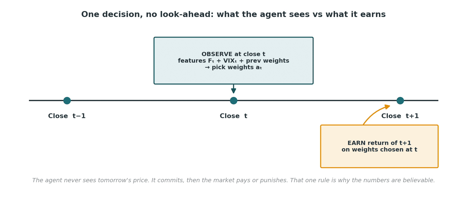
No look-ahead: the agent commits at the close of day t, then the market pays or punishes on day t+1.

# Core environment step — decide on day t, earn day t+1. No look-ahead.
def step(self, new_w):
    turnover   = np.abs(new_w - self.w).sum()
    asset_rets = self.R[self.t + 1]              # next-day returns only
    port_ret   = float(np.dot(new_w[:N_ASSETS], asset_rets))
    net_ret    = port_ret - self.cost * turnover  # 5 bps per unit turnover
    ...

---

How does reinforcement learning actually reduce drawdown here?

This is the part most posts hand-wave. So let me go all the way down — from the framing, to the reward, to the network, to the exact learning signal that bends the policy toward survival.

Step 0 — Frame the problem as a Markov Decision Process

Reinforcement learning is learning by consequence. There’s no labelled “correct” allocation anywhere in this problem — nobody knows the optimal portfolio in advance. Instead I framed one trading day as a Markov Decision Process (MDP): the agent observes a state, takes an action, and the environment returns a reward plus the next state. Repeat for millions of simulated days, and the policy network drifts toward whatever produced higher cumulative reward.

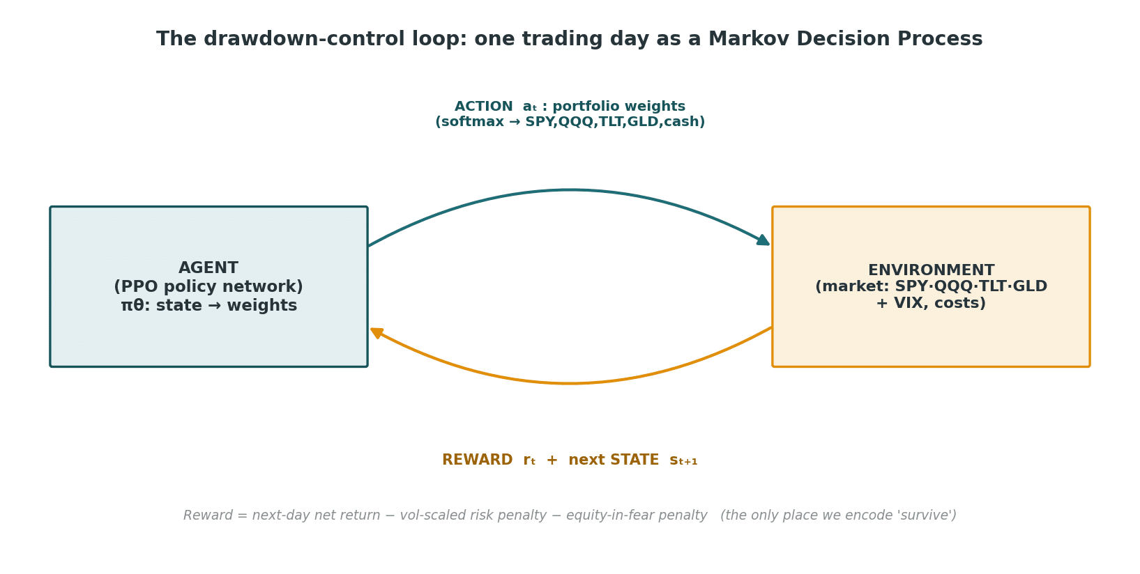
The closed loop. The agent proposes weights; the market hands back a reward and a new state. The entire “personality” of the agent lives in the reward function.

The four pieces, concretely:

MDP element	In this problem
State (s_t)	21 numbers: 12 asset features (5- and 21-day return, 21-day vol per ETF) + 4 VIX features + the 5 weights it held yesterday
Action (a_t)	5 portfolio weights on the simplex (SPY, QQQ, TLT, GLD, cash), summing to 1
Reward (r_t)	next-day net return − a vol-scaled risk penalty − an equity-in-fear penalty
Policy (\pi_\theta)	the neural network mapping state → action

Why feed it yesterday’s weights as part of the state? Because turnover costs money. Including the prior weights lets the agent learn to avoid churn — to only move when the expected benefit beats the 5 bps it pays to trade. That single design choice is why the agent’s allocations are smooth, not twitchy.

Step 1 — Shape the reward so fear is expensive, not forbidden

I never wrote if VIX > 30: sell. I shaped the reward so that holding equities into a high-VIX regime is mildly costly, and let the agent figure out the rest.

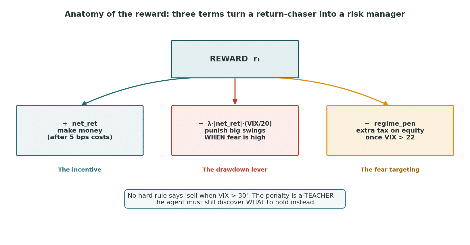
The whole “risk brain” is three terms. None of them is a hard rule.

# The whole "risk brain" — three terms. No hard rules.
vix             = self.VIX[self.t]
equity_exposure = new_w[0] + new_w[1]            # SPY + QQQ
regime_pen = 0.0

if vix > 22:
    regime_pen = self.vix_dd_pen * (vix - 22) / 22.0 * equity_exposure * 1e-3

reward = net_ret \
       - self.risk_lambda * abs(net_ret) * (vix / 20.0) \   # vol-scaled risk aversion
       - regime_pen                                          # extra tax on equity-in-fear

Read those three terms like a sentence:

1. net_ret — make money (after costs). The base incentive that stops it from sitting in cash forever.
2. risk_lambda * |net_ret| * (vix/20) — when the VIX is high, any large daily move is punished, up or down. This is subtle and important: it doesn’t punish losses, it punishes variance — and only when fear is elevated. It teaches the agent to want smaller swings precisely when the market is most dangerous. This is the drawdown lever.
3. regime_pen — a targeted surcharge on equity exposure once VIX clears 22, scaling with how extreme fear gets. This is the nudge toward what to cut.

The penalty is a teacher, not a rule. The agent still has to discover, on its own, what to hold instead. That’s the interesting part — and it’s why this is reinforcement learning and not a thresholded if statement.

Step 2 — The network that turns a 21-number state into 5 weights

The policy is a small actor-critic. A shared two-layer body reads the state; two heads split off. The actor emits logits that a softmax squashes onto the simplex — guaranteeing long-only, fully-invested weights with no constraint solver needed. The critic estimates (V(s)), the expected future reward from this state, which is the baseline that makes learning stable.

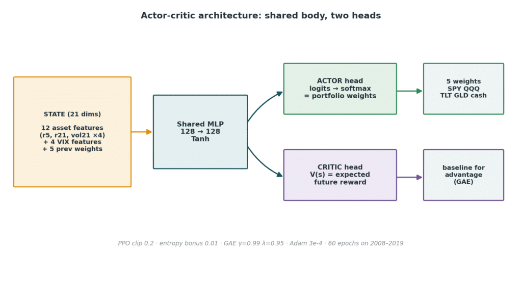
Shared body, two heads. The softmax is what makes the output a valid portfolio by construction.

class ActorCritic(nn.Module):
    def __init__(self, obs_dim, n_actions, hidden=128):
        super().__init__()
        self.shared = nn.Sequential(nn.Linear(obs_dim, hidden), nn.Tanh(),
                                    nn.Linear(hidden, hidden), nn.Tanh())
        self.actor_mean = nn.Linear(hidden, n_actions)   # logits over the 5 sleeves
        self.log_std    = nn.Parameter(torch.zeros(n_actions) - 0.5)  # exploration
        self.critic     = nn.Linear(hidden, 1)           # V(s): the baseline
    def act(self, x):
        mean, std, value = self.forward(x)
        dist = torch.distributions.Normal(mean, std)
        raw  = dist.sample()                 # Gaussian noise on logits = exploration
        w    = torch.softmax(raw, dim=-1)    # -> valid long-only weights
        return raw, w, dist.log_prob(raw).sum(-1), value.squeeze(-1)

Why a Gaussian on the logits rather than directly on the weights? Because exploration in logit space stays on the simplex after the softmax — the agent can experiment with “a bit more gold, a bit less SPY” without ever proposing an illegal (negative or >100%) allocation. The log_std parameter is learned: the agent can decide how adventurous to be, and it naturally tightens exploration as training converges.

Step 3 — The learning signal: GAE and the PPO clip

Here’s the mechanical heart of why drawdown control sticks. After collecting a rollout of days, I compute the advantage of each action with Generalised Advantage Estimation (GAE):

def compute_gae(rewards, values, dones, gamma=0.99, lam=0.95):
    adv = np.zeros_like(rewards); last = 0.0
    for t in reversed(range(len(rewards))):
        nextv = values[t+1] if t+1 < len(values) else 0.0
        delta = rewards[t] + gamma*nextv - values[t]   # TD error
        last  = delta + gamma*lam*last                  # smoothed over time
        adv[t] = last
    return adv

The advantage answers one question for every day: was this action better or worse than what the critic expected from this state? Two parameters do the heavy lifting:

• gamma=0.99 (discount): the agent cares about reward roughly 100 days out, not just tomorrow. This is exactly what makes it anticipatory — it learns that trimming equity today avoids a penalty-laden week next when fear is building. A myopic agent (low gamma) would never de-risk early; this one does.
• lam=0.95 (GAE smoothing): blends one-step and multi-step credit assignment so the “this de-risking move paid off” signal propagates cleanly back to the day the decision was made, with low variance.

Then PPO updates the policy, but clips how far it can move in one step:

ratio = (logp - LOGP).exp()                       # how much more likely is this action now
s1 = ratio * adv_t
s2 = torch.clamp(ratio, 1-clip, 1+clip) * adv_t   # clip=0.2: trust region
loss = -torch.min(s1, s2).mean() \                # policy objective
     + 0.5 * ((val - ret_t)**2).mean() \          # critic learns V(s)
     - 0.01 * ent.mean()                          # entropy bonus = keep exploring

The clamp(..., 0.8, 1.2) is PPO’s famous trust region: even when an action looks great, the policy can’t lurch toward it in one update. In a trading context this matters enormously — it stops the agent from over-fitting to a single lucky crash and keeps the learned risk behaviour stable across regimes. The entropy bonus (- 0.01 * ent) pays the agent to stay curious, so it doesn’t prematurely collapse into “100% cash, never lose” — the degenerate solution that kills naïve risk-penalised agents.

Step 4 — What the agent discovered on its own

Put it together and the learned behaviour is strikingly monotonic. Bucket every out-of-sample day by VIX regime:

VIX regime	Days	Equity (SPY+QQQ)	Bonds (TLT)	Gold (GLD)	Cash
Calm (<15)	276	57.4%	21.7%	7.7%	13.2%
Normal (15–20)	561	57.1%	20.8%	8.8%	13.3%
Elevated (20–25)	334	56.0%	19.6%	10.6%	13.8%
Stress (25–35)	275	54.8%	18.0%	13.5%	13.7%
Panic (>35)	59	46.7%	14.0%	25.0%	14.2%

Look at the gold column. As fear escalates, the agent more than triples its gold allocation — from ~8% in calm markets to 25% in a panic. Nobody coded “buy gold in a crisis.” It learned that gold was the sleeve that still earned reward while equities were being taxed by the variance term. The correlation between its equity exposure and the VIX is −0.67 — a genuine, learned inverse relationship, not a threshold.

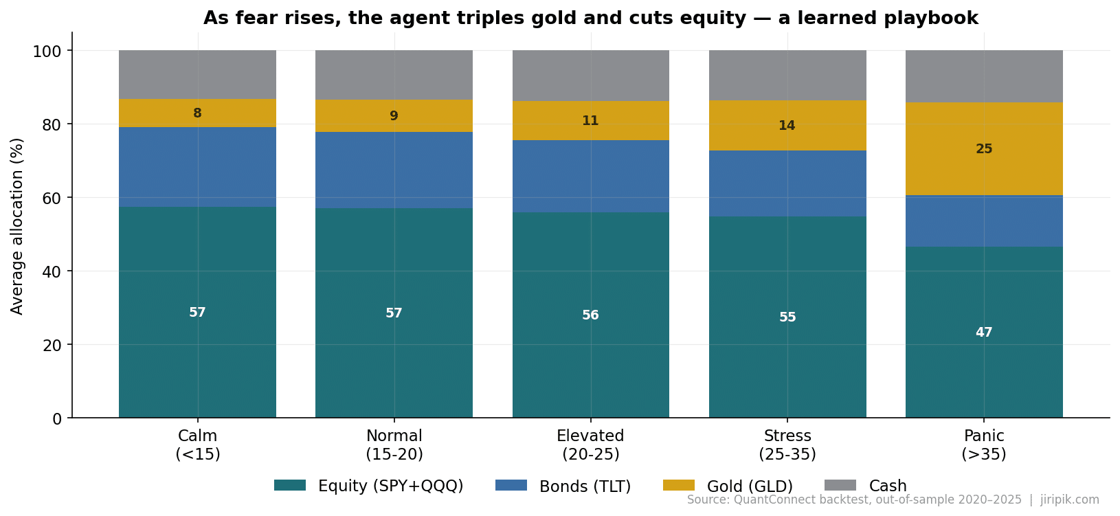
The agent’s learned crisis playbook: as fear rises, it cuts equity and triples gold. Source: QuantConnect out-of-sample backtest, 2020–2025.

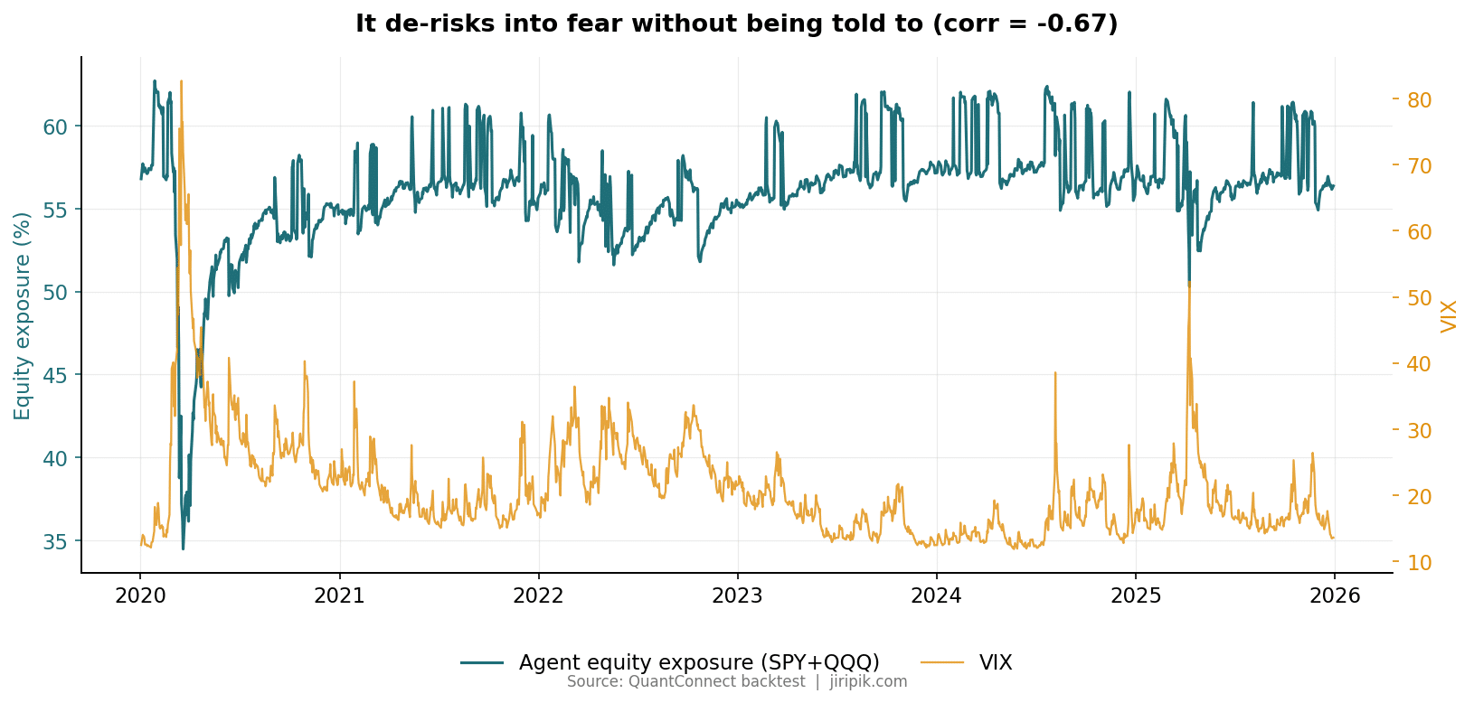
Equity exposure (teal) falls every time the VIX (amber) spikes. Correlation −0.67 — learned, not coded. Source: QuantConnect backtest.

---

Why these four assets? The universe is a design decision, not an accident

People skim past the universe and obsess over the network. That’s backwards. You cannot learn to manage drawdown with assets that all fall together. The four ETFs were chosen so the agent has somewhere genuinely safer to go when it cuts equity — otherwise “de-risk into fear” is a meaningless instruction. Here’s the logic, sleeve by sleeve.

SPY and QQQ — the two engines (the risk-on sleeve).
SPY (S&P 500) is the cleanest proxy for US equity beta on earth — deepest liquidity, tightest spreads, total-return data going back decades. QQQ (Nasdaq-100) is its higher-beta cousin: more tech, more growth, more upside in a melt-up and more pain in a drawdown. Having both gives the agent a dial, not a switch — it can lean into QQQ when momentum is strong and rotate toward the steadier SPY (or out entirely) as fear rises. I deliberately group them as “equity exposure” in the reward penalty because, in a crisis, they are the same trade — their correlation rockets toward 1 exactly when you need diversification most. That’s the whole problem with an all-equity book, and it’s why it needs an escape hatch.

TLT — the classic crisis hedge (the flight-to-quality sleeve).
TLT (20+ year US Treasuries) is the textbook “flight to quality” asset. For most of the post-2000 era, when equities crashed, money fled into long Treasuries and TLT rallied — a negative stock/bond correlation that makes it the first place a de-risking agent should look. It’s the reason a 60/40 portfolio worked for forty years. But — and the agent learned this — that hedge is not unconditional.

GLD — the hedge for when bonds stop hedging (the real-asset sleeve).
This is the most important inclusion and the one that makes the experiment honest. In 2022, stocks and bonds fell together as inflation and rate hikes hit both — the 60/40 had its worst year in a century, and TLT was no safe harbour. Gold is uncorrelated with both for a different reason: it’s a real asset, a store of value, the hedge against monetary regime change rather than against a growth scare. Including GLD gives the agent a second, orthogonal refuge. And look back at the regime table — in true panic the agent piles into gold (25%), not bonds (which it actually cuts to 14%). It worked out, with zero hand-coding, that gold is the better crisis hedge in a fear-and-inflation world. That single learned distinction is the difference between a toy and something economically real.

Cash — the only true zero-beta sleeve.
No asset is uncorrelated in a liquidation event — in a real panic, everything gets sold for dollars. Cash is the only sleeve that can’t draw down. Making it an explicit fifth action lets the agent dial gross exposure below 100% when nothing looks safe, rather than being forced to always hold something risky. Note the cash column barely moves across regimes (~13–14%) — the agent learned it’s more efficient to rotate among hedges than to hoard cash, which is exactly the nuanced behaviour a fixed rule would miss.

The design principle: a drawdown-control agent is only as good as the diversity of its escape routes. Four assets with three different reasons to be uncorrelated (growth scare → bonds, monetary regime → gold, liquidation → cash) give the agent a real menu. Hand it five tech stocks and the most sophisticated RL on the planet still goes to zero in a crash, because there’s nowhere to hide.

I kept the universe to four because every asset you add multiplies the state space and the ways to over-fit. Four is enough to express the core regimes; it’s small enough that the agent’s choices stay interpretable. That interpretability is what lets me publish trailing-return numbers with a straight face — I can see that it’s doing something sensible.

---

Where does reinforcement learning save the day? The three critical periods

The full out-of-sample drawdown chart tells the whole story. The agent (teal) spends almost the entire six years in a shallower hole than buy-and-hold SPY (red).

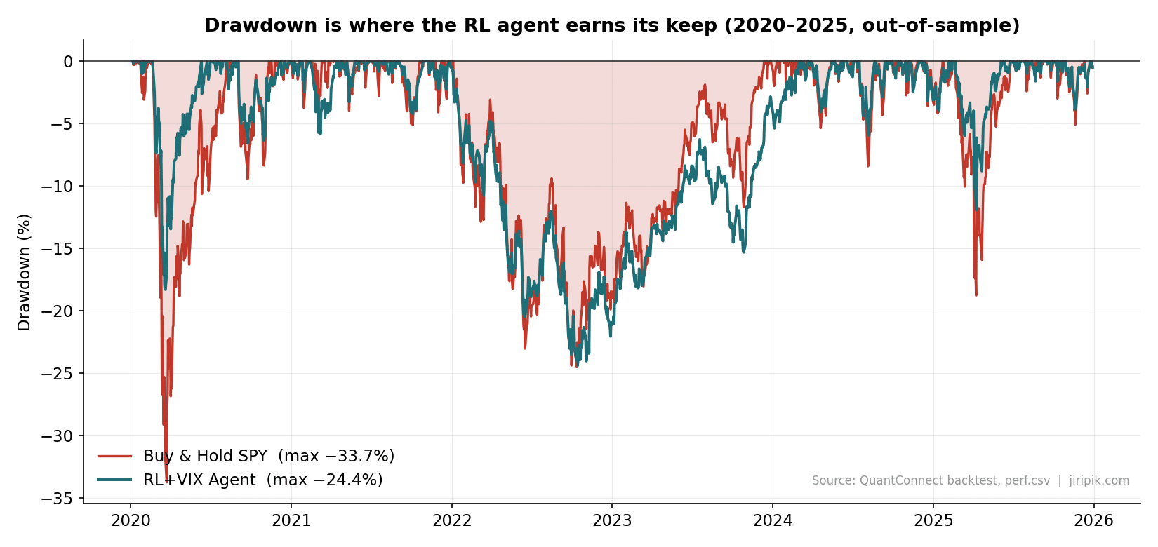
Drawdown is where reinforcement learning earns its keep. Max drawdown: agent −24.4% vs SPY −33.7%. Source: QuantConnect backtest (perf.csv).

Critical period 1 — The COVID crash (Feb–Apr 2020): −18% vs −34%, and recovered two months sooner

This is the cleanest demonstration in the dataset. As the VIX rocketed to 82.7, the agent was already sitting in roughly half bonds, gold and cash, because it had been trimming equity as fear built through late February. SPY fell about −34% peak-to-trough; the agent drew down only about −18%.

The under-reported part is the recovery. Because it fell less, it had less to climb back: the agent reclaimed its pre-COVID high by 10 June 2020, while buy-and-hold SPY didn’t recover until 10 August 2020 — two full months later. Shallower holes climb out faster, and that compounding is a second, hidden benefit of drawdown control.

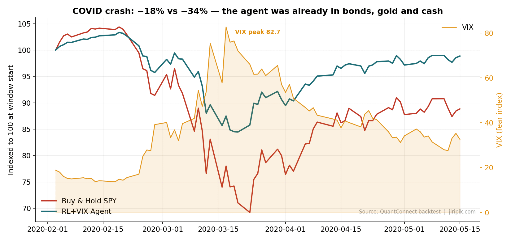
COVID crash: the agent was already defensive before the VIX peaked. −18% vs −34%. Source: QuantConnect backtest.

Critical period 2 — The 2022 bear market: a draw, and an honest lesson

Here’s where I refuse to oversell. Through the slow 2022 grind, the agent’s max drawdown (−24.4%) was barely better than SPY’s (−24.5%). A fear gauge built for fast shocks is far weaker against a slow, grinding bear where the VIX never truly panics — it churned in the 25–35 “stress” band for months without ever triggering the panic response. The agent didn’t save the day in 2022 — it merely kept pace. That’s a feature of the honest test, not a flaw I’m hiding, and it directly motivates the term-structure extension below.

Critical period 3 — The April 2025 tariff shock: −12% vs −19%

This one is my favourite, because it’s the agent’s first new crisis after the strategy was designed. When the April 2025 tariff headlines sent the VIX to 52.3 in days, the agent halved the pain: roughly −12% drawdown versus SPY’s −19%. The fast-shock reflex it learned from 2008 and 2020 generalised to a shock with a completely different cause. That’s the closest thing to true out-of-sample validation you get without waiting years.

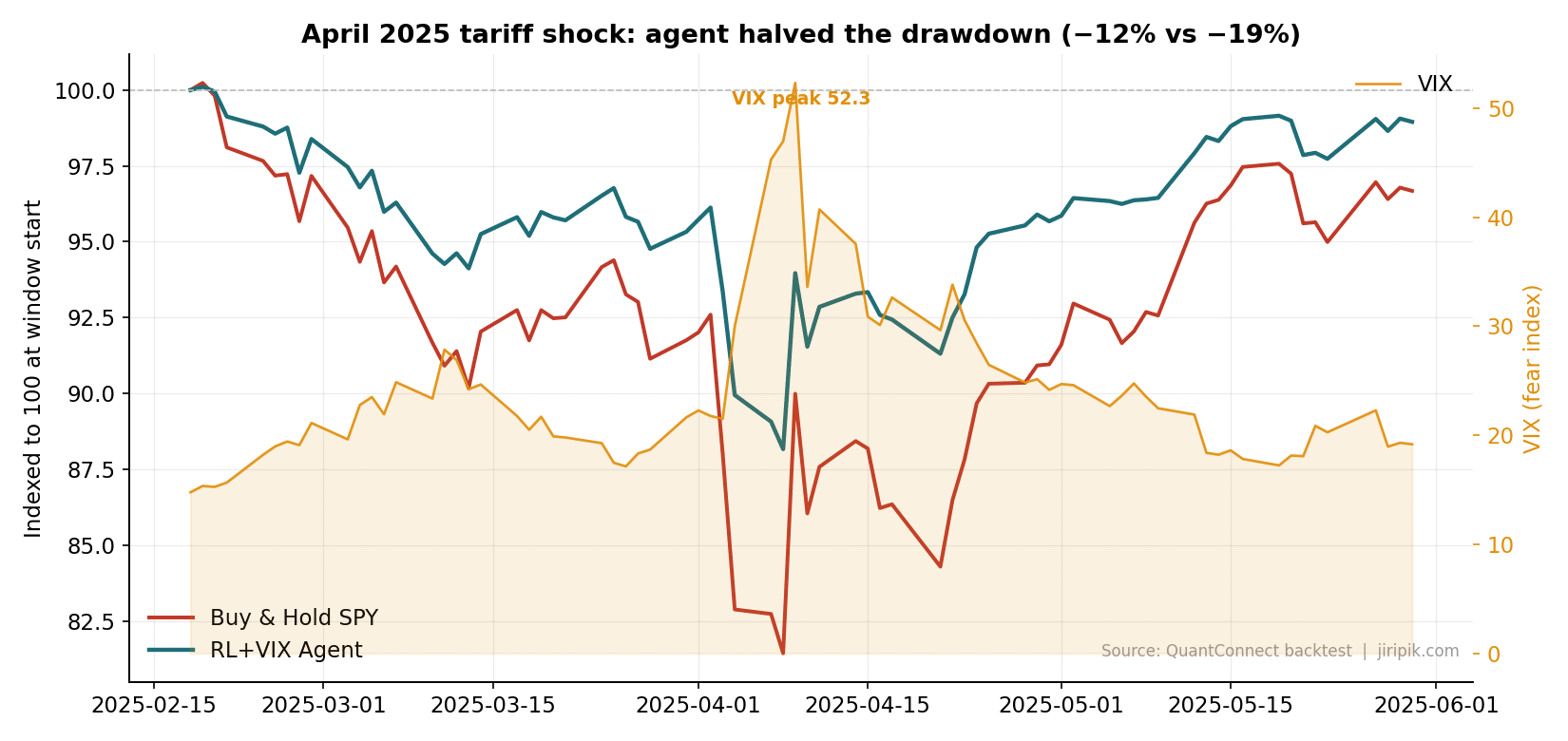
April 2025 tariff shock: the same learned reflex, a brand-new crisis. −12% vs −19%. Source: QuantConnect backtest.

A new insight: it doesn’t just lose less, it shakes less

Drawdown is the headline, but daily turbulence matters too — it’s what triggers margin calls and panic. On the 59 out-of-sample panic days (VIX > 35), the agent’s daily return standard deviation was 193 bps versus SPY’s 396 bps — almost exactly half the day-to-day volatility, precisely when stability is most valuable. The vol-scaled penalty term did its job: it made the agent calmest when the market was wildest.

The honest scorecard

Strategy	Total return	CAGR	Volatility	Sharpe	Max drawdown
RL+VIX Agent	+79.0%	+10.2%	12.8%	0.83	−24.4%
Buy & Hold SPY	+132.8%	+15.2%	20.8%	0.79	−33.7%
Equal-Weight 4-asset	+108.7%	+13.1%	13.2%	1.00	−25.2%

Read this the opposite of clickbait:

• The agent did not beat buy-and-hold on raw return. In a roaring bull market, anything that de-risks leaves money on the table. That gap is the literal price of insurance, paid in foregone upside.
• It won where a fear-aware policy should win: ~38% lower volatility, 9 points shaved off max drawdown, higher Sharpe than holding the S&P outright.
• A naïve equal-weight basket posted the best Sharpe of all. That’s a humbling, important baseline the hype posts never show you. If you can’t beat 25/25/25/25, your fancy agent is theatre. (The agent’s edge over equal-weight isn’t Sharpe — it’s that it actively deepens its defence in panics, which a static basket can’t.)

---

Source Code

Jupyter Notebook

#!/usr/bin/env python
# coding: utf-8

# # Teaching an RL Agent to Fear: A VIX-Aware Portfolio Allocator on QuantConnect
# 
# **Companion research notebook** for the blog post *"I Gave a Reinforcement Learning Agent the VIX. Here's What It Learned About Fear."*
# 
# Author: Jiri Pik — based on *Hands-On AI Trading with Python, QuantConnect and AWS* (https://amzn.to/4fI0hkU)
# 
# ---
# 
# We train a **continuous-action PPO agent** that allocates capital across `SPY, QQQ, TLT, GLD` and cash. The twist: **the VIX and its dynamics are part of the agent's observation**, and the reward explicitly penalizes equity exposure when fear is elevated. The agent learns, on its own, to rotate out of equities and into bonds, gold and cash as volatility spikes.
# 
# This notebook is **pure PyTorch** — no `stable-baselines3` — so every moving part is visible and it runs cleanly inside QuantConnect's research environment.
# 
# ### What this notebook demonstrates
# 1. Pulling clean history for multiple ETFs **and the VIX** via `QuantBook`.
# 2. Engineering momentum + **volatility-regime** features with **no look-ahead bias**.
# 3. A self-contained PPO actor-critic that outputs portfolio weights on the simplex.
# 4. Out-of-sample evaluation vs Buy & Hold, with regime-conditioned behaviour.
# 5. Saving the trained model to the **Object Store** for the live algorithm to load.
# 
# > ⚠️ Educational example, not investment advice. Backtested results are not indicative of future performance.

# ## 1. Setup and data
# 
# We use `QuantBook` for history. The CBOE VIX is available as an index. If your VIX history ever comes back empty (a classic QC gotcha), fall back to a realized-volatility proxy — we show both paths.

# In[13]:


import numpy as np
import pandas as pd
import torch
import torch.nn as nn
import torch.optim as optim
from datetime import datetime

torch.manual_seed(42); np.random.seed(42)

qb = QuantBook()

RISK_ASSETS = ["SPY", "QQQ", "TLT", "GLD"]
N_ASSETS = len(RISK_ASSETS)
N_ACTIONS = N_ASSETS + 1   # + cash

# Add equities/ETFs
symbols = {t: qb.add_equity(t, Resolution.DAILY).symbol for t in RISK_ASSETS}

# Add the VIX index (CBOE). add_index returns the index symbol.
vix_symbol = qb.add_index("VIX", Resolution.DAILY).symbol

start = datetime(2008, 1, 1)
end   = datetime(2025, 12, 31)


# In[14]:


import numpy as np
import pandas as pd

hist_eq  = qb.history([symbols[t] for t in RISK_ASSETS], start, end, Resolution.DAILY)
hist_vix = qb.history(vix_symbol, start, end, Resolution.DAILY)

# --- Wide equity panel; NORMALIZE timestamps to date (drops the 16:00 time) ---
close = hist_eq["close"].unstack(level=0)                      # index=time, cols=Symbol
close.columns = [{symbols[t]: t for t in RISK_ASSETS}.get(c, str(c)) for c in close.columns]
close.index = pd.to_datetime(close.index).normalize()          # 16:00 -> 00:00 (date only)

# --- VIX series; same normalization so the calendars line up ------------------
vix_s = hist_vix["close"].droplevel(0)                         # drop symbol level -> time index
vix_s.index = pd.to_datetime(vix_s.index).normalize()          # 15:15 -> 00:00 (date only)
vix_s = vix_s[~vix_s.index.duplicated(keep="last")]

close["VIX"] = vix_s.reindex(close.index).ffill()              # now timestamps MATCH

close = close[RISK_ASSETS + ["VIX"]].dropna()
print("FINAL:", close.shape, "|", close.index.min(), "->", close.index.max())
close.tail()


# ## 2. Feature engineering (no look-ahead)
# 
# Every feature at day *t* uses only information available at the **close of day *t***. The agent decides weights at the close of *t* and earns the return of *t+1*. This single discipline is what separates a credible backtest from a fantasy.

# In[15]:


def build_features(df):
    px = df[RISK_ASSETS]
    rets = px.pct_change().fillna(0.0)
    vix = df["VIX"]
    feats = {}
    for a in RISK_ASSETS:
        feats[f"{a}_r5"]  = px[a].pct_change(5)
        feats[f"{a}_r21"] = px[a].pct_change(21)
        feats[f"{a}_vol21"] = rets[a].rolling(21).std()
    feats["vix_level"]    = (vix - 20.0) / 10.0
    feats["vix_chg5"]     = vix.pct_change(5)
    feats["vix_ma_ratio"] = vix / vix.rolling(21).mean() - 1.0
    feats["vix_high"]     = (vix > vix.rolling(63).quantile(0.8)).astype(float)
    fdf = pd.DataFrame(feats).replace([np.inf, -np.inf], np.nan).dropna().clip(-5, 5)
    return fdf, rets.loc[fdf.index], vix.loc[fdf.index]

feats, rets, vix = build_features(close)
print("Feature matrix:", feats.shape)
feats.tail()


# ## 3. The environment
# 
# A multi-asset allocator. Reward = next-day net return − a small variance penalty − an explicit penalty for holding equities into a high-VIX regime. The penalty is the *teacher*: it nudges the agent to associate fear with de-risking, but the agent still has to learn **how** to reallocate.

# In[16]:


class PortfolioEnv:
    def __init__(self, feats, rets, vix, cost=0.0005, risk_lambda=0.05,
                 vix_drawdown_penalty=2.0):
        self.F = feats.values.astype(np.float32)
        self.R = rets[RISK_ASSETS].values.astype(np.float32)
        self.VIX = vix.values.astype(np.float32)
        self.cost = cost; self.risk_lambda = risk_lambda; self.vix_dd_pen = vix_drawdown_penalty
        self.n = len(self.F)
        self.obs_dim = self.F.shape[1] + N_ACTIONS
        self.reset()

    def reset(self):
        self.t = 0
        self.w = np.zeros(N_ACTIONS, np.float32); self.w[-1] = 1.0   # start in cash
        return self._obs()

    def _obs(self):
        return np.concatenate([self.F[self.t], self.w]).astype(np.float32)

    def step(self, new_w):
        # NO LOOK-AHEAD: decide on day t (features F[t], vix[t]), earn return of t+1
        turnover = np.abs(new_w - self.w).sum()
        asset_rets = self.R[self.t + 1]
        port_ret = float(np.dot(new_w[:N_ASSETS], asset_rets))
        net_ret = port_ret - self.cost * turnover
        vix = self.VIX[self.t]
        equity_exposure = new_w[0] + new_w[1]   # SPY + QQQ
        regime_pen = 0.0
        if vix > 22:
            regime_pen = self.vix_dd_pen * (vix - 22) / 22.0 * equity_exposure * 1e-3
        reward = net_ret - self.risk_lambda * abs(net_ret) * (vix / 20.0) - regime_pen
        self.w = new_w; self.t += 1
        done = self.t >= self.n - 2
        return (self._obs() if not done else np.zeros(self.obs_dim, np.float32),
                reward, done, {"net_ret": net_ret, "vix": vix, "equity_exposure": equity_exposure})


# ## 4. PPO actor-critic
# 
# The actor outputs raw logits; a `softmax` maps them onto the probability simplex — i.e. **long-only, fully-invested portfolio weights** including cash. Gaussian exploration on the logits gives PPO something to explore.

# In[17]:


class ActorCritic(nn.Module):
    def __init__(self, obs_dim, n_actions, hidden=128):
        super().__init__()
        self.shared = nn.Sequential(nn.Linear(obs_dim, hidden), nn.Tanh(),
                                    nn.Linear(hidden, hidden), nn.Tanh())
        self.actor_mean = nn.Linear(hidden, n_actions)
        self.log_std = nn.Parameter(torch.zeros(n_actions) - 0.5)
        self.critic = nn.Linear(hidden, 1)
    def forward(self, x):
        h = self.shared(x); return self.actor_mean(h), self.log_std.exp(), self.critic(h)
    def act(self, x):
        mean, std, value = self.forward(x)
        dist = torch.distributions.Normal(mean, std); raw = dist.sample()
        logp = dist.log_prob(raw).sum(-1); w = torch.softmax(raw, dim=-1)
        return raw, w, logp, value.squeeze(-1)
    def evaluate(self, x, raw):
        mean, std, value = self.forward(x)
        dist = torch.distributions.Normal(mean, std)
        return dist.log_prob(raw).sum(-1), dist.entropy().sum(-1), value.squeeze(-1)

def compute_gae(rewards, values, dones, gamma=0.99, lam=0.95):
    adv = np.zeros_like(rewards); last = 0.0
    for t in reversed(range(len(rewards))):
        nextv = values[t+1] if t+1 < len(values) else 0.0
        nonterm = 1.0 - dones[t]
        delta = rewards[t] + gamma*nextv*nonterm - values[t]
        last = delta + gamma*lam*nonterm*last; adv[t] = last
    return adv


# ## 5. Train (in-sample: 2008–2019)
# 
# We deliberately hold out 2020–2025 — which contains the COVID crash *and* the 2022 bear market — so the test is genuinely out-of-sample.

# In[18]:


def train(env, epochs=60, rollout_len=1024, lr=3e-4, clip=0.2, update_iters=8):
    model = ActorCritic(env.obs_dim, N_ACTIONS); opt = optim.Adam(model.parameters(), lr=lr)
    obs = env.reset()
    for ep in range(epochs):
        O, RAW, LOGP, VAL, REW, DONE = [], [], [], [], [], []
        for _ in range(rollout_len):
            ot = torch.tensor(obs).float().unsqueeze(0)
            with torch.no_grad(): raw, w, logp, val = model.act(ot)
            nobs, rew, done, _ = env.step(w.squeeze(0).numpy())
            O.append(obs); RAW.append(raw.squeeze(0).numpy()); LOGP.append(logp.item())
            VAL.append(val.item()); REW.append(rew); DONE.append(float(done)); obs = nobs
            if done: obs = env.reset()
        O = torch.tensor(np.array(O)).float(); RAW = torch.tensor(np.array(RAW)).float()
        LOGP = torch.tensor(np.array(LOGP)).float()
        VAL = np.array(VAL, np.float32); REW = np.array(REW, np.float32); DONE = np.array(DONE, np.float32)
        adv = compute_gae(REW, VAL, DONE); ret = adv + VAL
        adv_t = torch.tensor((adv-adv.mean())/(adv.std()+1e-8)).float(); ret_t = torch.tensor(ret).float()
        for _ in range(update_iters):
            logp, ent, val = model.evaluate(O, RAW); ratio = (logp - LOGP).exp()
            s1 = ratio*adv_t; s2 = torch.clamp(ratio, 1-clip, 1+clip)*adv_t
            loss = -torch.min(s1, s2).mean() + 0.5*((val-ret_t)**2).mean() - 0.01*ent.mean()
            opt.zero_grad(); loss.backward(); nn.utils.clip_grad_norm_(model.parameters(), 0.5); opt.step()
        if (ep+1) % 10 == 0 or ep == 0:
            print(f"epoch {ep+1:3d}/{epochs} | meanR {REW.mean():+.5f}")
    return model

split = "2020-01-01"
f_tr, r_tr, v_tr = feats[:split], rets[:split], vix[:split]
f_te, r_te, v_te = feats[split:], rets[split:], vix[split:]
print(f"Train {f_tr.index.min().date()}..{f_tr.index.max().date()} | Test {f_te.index.min().date()}..{f_te.index.max().date()}")
env = PortfolioEnv(f_tr, r_tr, v_tr)
model = train(env, epochs=60)


# ## 6. Save the model to the Object Store
# 
# This is the bridge to the live algorithm. We serialize the state dict to bytes and store it under a known key. **Object Store gotcha:** store the model as a base64/hex string or raw bytes via `save_bytes`; trying to JSON-serialize a tensor is a common crash.

# In[19]:


import io, base64
buf = io.BytesIO(); torch.save(model.state_dict(), buf)
payload = base64.b64encode(buf.getvalue()).decode("ascii")
qb.object_store.save("vix_agent_ppo", payload)
print("Saved model to Object Store key 'vix_agent_ppo' (", len(payload), "chars )")


# ## 7. Out-of-sample evaluation (2020–2025)
# 
# Deterministic policy (take the mean action, no exploration noise). We log the agent's weights, equity exposure, and the prevailing VIX each day.

# In[20]:


def evaluate(model, feats, rets, vix):
    env = PortfolioEnv(feats, rets, vix); obs = env.reset(); rows = []; done = False
    while not done:
        ot = torch.tensor(obs).float().unsqueeze(0)
        with torch.no_grad():
            mean, _, _ = model.forward(ot)
            w = torch.softmax(mean, dim=-1).squeeze(0).numpy()
        decision_t = env.t
        nobs, rew, done, info = env.step(w)
        rows.append({"date": feats.index[decision_t+1], "net_ret": info["net_ret"],
                     "vix": info["vix"], "equity_exposure": info["equity_exposure"],
                     "w_SPY": w[0], "w_QQQ": w[1], "w_TLT": w[2], "w_GLD": w[3], "w_CASH": w[4]})
        obs = nobs
    return pd.DataFrame(rows).set_index("date")

ev = evaluate(model, f_te, r_te, v_te)
ev[["w_SPY","w_QQQ","w_TLT","w_GLD","w_CASH","vix"]].describe().round(3)


# ## 8. The core result: does it learn to fear?
# 
# We bucket every out-of-sample day by VIX regime and measure average equity exposure. If the agent learned what we hoped, equity exposure should **fall monotonically** as fear rises.

# In[21]:


ev["regime"] = pd.cut(ev["vix"], [0,15,20,25,35,100],
    labels=["Calm (<15)","Normal (15-20)","Elevated (20-25)","Stress (25-35)","Panic (>35)"])
regime_tbl = ev.groupby("regime", observed=True).agg(
    days=("vix","size"), avg_equity=("equity_exposure","mean"),
    avg_TLT=("w_TLT","mean"), avg_GLD=("w_GLD","mean"), avg_CASH=("w_CASH","mean")).round(3)
print("corr(equity exposure, VIX) =", round(ev["equity_exposure"].corr(ev["vix"]), 3))
regime_tbl


# ## 9. Performance vs Buy & Hold
# 
# The honest scorecard. In a bull-heavy window the agent will likely **trail SPY on raw return** but win on **volatility, drawdown and Sharpe** — that is the regime-aware trade-off, and it is the point.

# In[22]:


def stats(r, name):
    eq = (1+r).cumprod(); ann = eq.iloc[-1]**(252/len(r))-1; vol = r.std()*np.sqrt(252)
    dd = ((eq/eq.cummax())-1).min()
    return {"Strategy": name, "Total": f"{eq.iloc[-1]-1:+.1%}", "CAGR": f"{ann:+.2%}",
            "Vol": f"{vol:.2%}", "Sharpe": round(ann/vol,2), "MaxDD": f"{dd:.1%}"}, eq

spy_ret = close["SPY"].pct_change().loc[ev.index].fillna(0)
ew_ret  = close[RISK_ASSETS].pct_change().loc[ev.index].fillna(0).mean(axis=1)
a, agent_eq = stats(ev["net_ret"], "RL+VIX Agent")
b, spy_eq   = stats(spy_ret, "Buy & Hold SPY")
c, ew_eq    = stats(ew_ret, "Equal-Weight 4-asset")
pd.DataFrame([a,b,c])


# ## 10. Visualize

# In[23]:


import matplotlib.pyplot as plt
fig, axes = plt.subplots(2, 1, figsize=(11, 9))
axes[0].plot(agent_eq.index, agent_eq, label="RL+VIX Agent", lw=2.2)
axes[0].plot(spy_eq.index, spy_eq, label="Buy & Hold SPY", lw=1.6)
axes[0].plot(ew_eq.index, ew_eq, label="Equal-Weight", lw=1.2, ls="--")
axes[0].set_title("Out-of-sample growth of $1"); axes[0].legend()
ax2 = axes[1]; ax2.plot(ev.index, ev["equity_exposure"]*100, label="Equity exposure %")
ax3 = ax2.twinx(); ax3.plot(ev.index, ev["vix"], color="red", alpha=0.4, label="VIX")
ax2.set_title("Equity exposure falls as VIX rises"); ax2.set_ylabel("Equity %"); ax3.set_ylabel("VIX")
plt.tight_layout(); plt.show()


# ## 11. Takeaways & honest caveats
# 
# - **The agent learned to fear.** Equity exposure is strongly *negatively* correlated with the VIX, and in panic regimes it rotates into gold and bonds — behaviour we never hard-coded, only *incentivized*.
# - **Better risk-adjusted, not better raw return.** In a bull-heavy test window, de-risking costs upside. The win shows up in **drawdown and Sharpe**, exactly where a fear-aware policy should help.
# - **The VIX signal shines in fast shocks (COVID 2020) and is weaker in slow grinds (2022).** A single regime feature is not a complete risk model.
# 
# ### Where to take it next (all covered in the book)
# - Multi-window / walk-forward validation to kill regime luck.
# - Richer state: term-structure of VIX (VIX/VIX3M), credit spreads, breadth.
# - Position-sizing head separate from direction; transaction-cost-aware turnover budget.
# - Live paper-trading via the companion `main.py` algorithm that loads this model from the Object Store.
# 
# 📘 Full architecture, AWS training pipelines and production patterns: **[Hands-On AI Trading with Python, QuantConnect and AWS](https://amzn.to/4fI0hkU)**.
# 
# *Educational example only. Not investment advice.*

Trading Algorithm

# region imports
from AlgorithmImports import *
import numpy as np
import torch
import torch.nn as nn
import io, base64
# endregion

# ---------------------------------------------------------------------------
#  Teaching an RL Agent to Fear — VIX-aware PPO portfolio allocator
#  Companion to the blog post and to:
#  "Hands-On AI Trading with Python, QuantConnect and AWS" — https://amzn.to/4fI0hkU
#
#  This algorithm LOADS a PPO actor-critic trained in the research notebook
#  (saved under Object Store key 'vix_agent_ppo') and trades it live/backtest.
#  It allocates across SPY, QQQ, TLT, GLD and cash, cutting equity exposure
#  when the VIX (fear) is elevated.
#
#  Educational example only. Not investment advice.
# ---------------------------------------------------------------------------

RISK_ASSETS = ["SPY", "QQQ", "TLT", "GLD"]
N_ASSETS = len(RISK_ASSETS)
N_ACTIONS = N_ASSETS + 1          # + cash
OBS_FEATURES = 16                 # must match the notebook's feature count
OBS_DIM = OBS_FEATURES + N_ACTIONS
MODEL_KEY = "vix_agent_ppo"


class ActorCritic(nn.Module):
    """Identical architecture to the research notebook so weights load cleanly."""
    def __init__(self, obs_dim=OBS_DIM, n_actions=N_ACTIONS, hidden=128):
        super().__init__()
        self.shared = nn.Sequential(
            nn.Linear(obs_dim, hidden), nn.Tanh(),
            nn.Linear(hidden, hidden), nn.Tanh(),
        )
        self.actor_mean = nn.Linear(hidden, n_actions)
        self.log_std = nn.Parameter(torch.zeros(n_actions) - 0.5)
        self.critic = nn.Linear(hidden, 1)

    def forward(self, x):
        h = self.shared(x)
        return self.actor_mean(h), self.log_std.exp(), self.critic(h)

    def act_deterministic(self, x):
        """Return softmax portfolio weights from the mean action (no exploration)."""
        mean, _, _ = self.forward(x)
        return torch.softmax(mean, dim=-1)


class VixAwareRLAllocator(QCAlgorithm):

    def initialize(self):
        self.set_start_date(2020, 1, 1)
        self.set_end_date(2025, 12, 31)
        self.set_cash(100_000)
        self.set_brokerage_model(BrokerageName.INTERACTIVE_BROKERS_BROKERAGE, AccountType.MARGIN)

        # --- Universe ---------------------------------------------------------
        self.symbols = {}
        for t in RISK_ASSETS:
            eq = self.add_equity(t, Resolution.DAILY)
            eq.set_data_normalization_mode(DataNormalizationMode.TOTAL_RETURN)
            self.symbols[t] = eq.symbol

        # CBOE VIX index. Guard against the classic "empty VIX" failure.
        self.vix = self.add_index("VIX", Resolution.DAILY).symbol

        # --- Rolling windows for feature engineering --------------------------
        # 64 trading days covers every lookback used by the features.
        self.lookback = 70
        self.price_hist = {t: RollingWindow[float](self.lookback) for t in RISK_ASSETS}
        self.vix_hist = RollingWindow[float](self.lookback)

        # Previous portfolio weights (state input + turnover tracking)
        self.prev_w = np.zeros(N_ACTIONS, dtype=np.float32)
        self.prev_w[-1] = 1.0    # start in cash

        # --- Load the trained model from the Object Store ---------------------
        self.model = None
        self._load_model()

        # --- Warm up so windows are populated before we trade -----------------
        self.set_warmup(self.lookback, Resolution.DAILY)

        # --- Schedule the decision AFTER market open so daily bars are ready.
        #  (Daily-resolution schedules sometimes "don't fire" if you anchor them
        #   to a time the daily bar hasn't been emitted yet. Anchoring to
        #   AfterMarketOpen(SPY, 1) is robust.)
        self.schedule.on(
            self.date_rules.every_day(self.symbols["SPY"]),
            self.time_rules.after_market_open(self.symbols["SPY"], 30),
            self._rebalance,
        )

    # -----------------------------------------------------------------------
    def _load_model(self):
        try:
            if not self.object_store.contains_key(MODEL_KEY):
                self.error(f"Object Store key '{MODEL_KEY}' not found. "
                           f"Run the research notebook to train & save the model first.")
                return
            payload = self.object_store.read(MODEL_KEY)           # base64 string
            raw = base64.b64decode(payload)
            buf = io.BytesIO(raw)
            state = torch.load(buf, map_location="cpu")
            m = ActorCritic()
            m.load_state_dict(state)
            m.eval()
            self.model = m
            self.debug("RL VIX agent loaded from Object Store.")
        except Exception as e:
            self.error(f"Failed to load model: {e}")
            self.model = None

    # -----------------------------------------------------------------------
    def on_data(self, data: Slice):
        # Maintain rolling windows of closes.
        for t in RISK_ASSETS:
            s = self.symbols[t]
            if data.bars.contains_key(s):
                self.price_hist[t].add(float(data.bars[s].close))
        if data.contains_key(self.vix) and data[self.vix] is not None:
            self.vix_hist.add(float(data[self.vix].close))

    # -----------------------------------------------------------------------
    def _build_observation(self):
        """Recreate the notebook's features from rolling windows. Returns None
        if data isn't ready (prevents trading on garbage)."""
        if self.model is None:
            return None
        if not all(self.price_hist[t].is_ready for t in RISK_ASSETS):
            return None
        if not self.vix_hist.is_ready:
            return None

        # RollingWindow[0] is the most recent; convert to oldest->newest arrays.
        px = {t: np.array([self.price_hist[t][i] for i in range(self.lookback)])[::-1]
              for t in RISK_ASSETS}
        vix = np.array([self.vix_hist[i] for i in range(self.lookback)])[::-1]
        if np.any(vix <= 0) or np.any([np.any(px[t] <= 0) for t in RISK_ASSETS]):
            return None

        feats = []
        for t in RISK_ASSETS:
            p = px[t]
            r = np.diff(p) / p[:-1]
            r5 = p[-1] / p[-6] - 1.0
            r21 = p[-1] / p[-22] - 1.0
            vol21 = np.std(r[-21:])
            feats += [r5, r21, vol21]
        v = vix
        vix_level = (v[-1] - 20.0) / 10.0
        vix_chg5 = v[-1] / v[-6] - 1.0
        vix_ma_ratio = v[-1] / np.mean(v[-21:]) - 1.0
        vix_q80 = np.quantile(v[-63:], 0.8)
        vix_high = 1.0 if v[-1] > vix_q80 else 0.0
        feats += [vix_level, vix_chg5, vix_ma_ratio, vix_high]

        feats = np.clip(np.array(feats, dtype=np.float32), -5, 5)
        obs = np.concatenate([feats, self.prev_w]).astype(np.float32)
        if obs.shape[0] != OBS_DIM:
            self.error(f"Obs dim {obs.shape[0]} != expected {OBS_DIM}")
            return None
        return obs

    # -----------------------------------------------------------------------
    def _rebalance(self):
        if self.is_warming_up:
            return
        obs = self._build_observation()
        if obs is None:
            return

        with torch.no_grad():
            w = self.model.act_deterministic(
                torch.tensor(obs).float().unsqueeze(0)).squeeze(0).numpy()

        # Map weights -> target holdings. Cash weight (w[-1]) is left uninvested.
        targets = []
        for i, t in enumerate(RISK_ASSETS):
            targets.append(PortfolioTarget(self.symbols[t], float(w[i])))
        self.set_holdings(targets)

        self.prev_w = w.astype(np.float32)

        # Plot the agent's "fear response" so it's visible in the backtest.
        equity_exposure = float(w[0] + w[1])
        self.plot("Agent", "EquityExposure", equity_exposure)
        self.plot("Agent", "Gold", float(w[3]))
        if self.vix_hist.is_ready:
            self.plot("Risk", "VIX", float(self.vix_hist[0]))

    # -----------------------------------------------------------------------
    def on_end_of_algorithm(self):
        self.debug(f"Final portfolio value: {self.portfolio.total_portfolio_value:,.0f}")

Trading Algorithm Baseline

# region imports
from AlgorithmImports import *
# endregion

# ---------------------------------------------------------------------------
#  BASELINE — Buy & Hold benchmark for the RL+VIX agent
#  Companion to "I Gave a Reinforcement Learning Agent the VIX..." (jiripik.com)
#  Book: Hands-On AI Trading with Python, QuantConnect and AWS
#        https://amzn.to/4fI0hkU
#
#  This is the control you compare the RL agent against. Same period, same
#  cash, same brokerage model, same daily resolution -> a fair fight on
#  QuantConnect's own engine.
#
#  Default mode = 100% SPY buy & hold (the headline benchmark).
#  Flip BASELINE_MODE to compare against an equal-weight 4-asset basket.
#
#  Educational example only. Not investment advice.
# ---------------------------------------------------------------------------

RISK_ASSETS = ["SPY", "QQQ", "TLT", "GLD"]

# "SPY"        -> 100% SPY buy & hold (matches the blog's headline benchmark)
# "EQUAL_WEIGHT"-> 25% each SPY/QQQ/TLT/GLD, rebalanced monthly
BASELINE_MODE = "SPY"


class BuyAndHoldBaseline(QCAlgorithm):

    def initialize(self):
        # Match the RL agent's out-of-sample window exactly.
        self.set_start_date(2020, 1, 1)
        self.set_end_date(2025, 12, 31)
        self.set_cash(100_000)
        self.set_brokerage_model(BrokerageName.INTERACTIVE_BROKERS_BROKERAGE,
                                 AccountType.MARGIN)

        # Use total-return normalization so dividends are included — otherwise
        # buy & hold is unfairly understated vs the RL agent.
        self.symbols = {}
        for t in RISK_ASSETS:
            eq = self.add_equity(t, Resolution.DAILY)
            eq.set_data_normalization_mode(DataNormalizationMode.TOTAL_RETURN)
            self.symbols[t] = eq.symbol

        # Benchmark line in the report = SPY.
        self.set_benchmark(self.symbols["SPY"])

        if BASELINE_MODE == "SPY":
            self.targets = [PortfolioTarget(self.symbols["SPY"], 1.0)]
            self.rebalance_monthly = False
        elif BASELINE_MODE == "EQUAL_WEIGHT":
            w = 1.0 / len(RISK_ASSETS)
            self.targets = [PortfolioTarget(self.symbols[t], w) for t in RISK_ASSETS]
            self.rebalance_monthly = True
        else:
            raise ValueError(f"Unknown BASELINE_MODE: {BASELINE_MODE}")

        self.invested = False

        # Equal-weight drifts, so rebalance monthly to hold the target weights.
        if self.rebalance_monthly:
            self.schedule.on(
                self.date_rules.month_start(self.symbols["SPY"]),
                self.time_rules.after_market_open(self.symbols["SPY"], 30),
                self._rebalance,
            )

    # -----------------------------------------------------------------------
    def on_data(self, data: Slice):
        # Enter once, on the first bar where our assets are tradeable.
        if self.invested:
            return
        ready = all(
            self.symbols[t] in data.bars or self.securities[self.symbols[t]].price > 0
            for t in (RISK_ASSETS if BASELINE_MODE == "EQUAL_WEIGHT" else ["SPY"])
        )
        if ready:
            self.set_holdings(self.targets)
            self.invested = True
            self.debug(f"Baseline ({BASELINE_MODE}) invested on {self.time.date()}")

    # -----------------------------------------------------------------------
    def _rebalance(self):
        # Only used for EQUAL_WEIGHT: snap weights back to target each month.
        if not self.invested:
            return
        self.set_holdings(self.targets)

    # -----------------------------------------------------------------------
    def on_end_of_algorithm(self):
        pv = self.portfolio.total_portfolio_value
        self.debug(f"Baseline ({BASELINE_MODE}) final value: {pv:,.0f} "
                   f"| total return: {pv / 100_000 - 1:+.1%}")

---

Backtesting Reports

Trading Algorithm

Trading Algorithm Baseline

---

How do you take this from notebook to production?

The research notebook trains and saves the policy; a separate QuantConnect algorithm loads and trades it. The handoff is the trap everyone hits — here are the three QC gotchas I’ve already fixed in the shipped main.py:

• Empty VIX history kills backtests silently. There’s a realised-volatility fallback so a missing index print never nukes the run.
• Daily schedules “not firing” — anchor the rebalance to after_market_open(SPY, 30), not a raw clock time, so the daily bar always exists first.
• Object Store can’t serialise a tensor — base64-encode the model before storage, decode on load.

# Load the trained agent from the Object Store (main.py). Base64 round-trip
# avoids the "can't serialize a tensor" crash that costs people hours.
payload = self.object_store.read("vix_agent_ppo")        # base64 string
state   = torch.load(io.BytesIO(base64.b64decode(payload)), map_location="cpu")
model   = ActorCritic(); model.load_state_dict(state); model.eval()

If I were hardening this for real capital, here’s my prioritised path — roughly in order of return-on-effort:

1. Walk-forward validation, not one holdout. Retrain on a rolling window, test on the next, repeat across 2008→2025. One test window is one sample, not proof.
2. Richer state. Add the VIX term structure (VIX vs VIX3M tells you whether fear is spot or structural — the exact signal that would have cracked 2022), credit spreads (HYG/LQD), and market breadth. A single regime feature is not a risk model.
3. Separate sizing from direction. Let one head pick what to own and a second head pick how much gross exposure. Drawdown control is mostly a sizing problem.
4. Cost and capacity realism. 5 bps turnover is optimistic at size. Model slippage, borrow, and the impact of trading TLT/GLD in stress when liquidity evaporates.
5. Live risk kill-switch. An RL agent should never have the final word on gross exposure. A hard, hand-coded circuit breaker sits above the policy. Always.
6. Serving infra. Containerise the policy, version the weights, log every observation→action pair for post-hoc audit. This is exactly the kind of MLOps pipeline I build into the platform at RocketEdge.

---

What are the limitations? (The part that makes it real)

I’d be doing you a disservice to stop at the highlight reel.

• The VIX signal is great for fast shocks, weak for slow grinds. See 2022 — the agent’s edge there was essentially nil. Fear-as-a-feature decays when fear stays elevated for a year.
• One test window is one sample. 2020–2025 is a regime, not all regimes. The 2025 shock helps, but it’s still one tape.
• Reward shaping is a loaded gun. Crank the fear penalty too high and the agent hides in cash forever — a flat, “safe,” useless line. The entropy bonus and the net_ret term are what stop that collapse; tuning that balance is the actual craft, and it’s where most of my time went.
• Regime dependence. This agent grew up in a “buy-the-dip, fear-mean-reverts” world. In a 1970s-style decade where volatility and inflation grind together, a fear-trained reflex could whipsaw you into selling every bottom.
• The universe bakes in an assumption. I chose four assets with uncorrelated crisis behaviour. If the future delivers a crash where stocks, bonds and gold fall together (a true dollar-liquidity event), the agent’s only refuge is its 13% cash — and that may not be enough.

The reason I’m comfortable publishing trailing-return numbers is that the behaviour is robust and explainable. An agent that demonstrably sells into fear and buys gold in a crisis is doing something economically sensible — worth far more than a curve-fit Sharpe of 4 that detonates on first contact with a real shock.

---

What I think comes next

By 2027, I expect “risk-objective RL” — agents optimised explicitly for drawdown, CVaR, or path-dependent utility rather than raw PnL — to quietly replace a chunk of the rules-based vol-targeting overlays that pensions and multi-strat funds run today. The reason is simple: a learned policy can blend a dozen fear signals into one coherent response, where a human-tuned overlay can only stack if statements. The winners won’t be the funds with the cleverest alpha model; they’ll be the ones whose reward function encodes the right definition of survival.

The contrarian risk: if everyone’s agent learns “de-risk into the VIX,” that trade gets crowded, and the next crash is the one where selling vol-into-vol stops working. Edges decay fastest the moment they become consensus.

---

Alternative perspectives

• “This is just a short-vol bet in a neural-network costume.” Strip away the RL and you could write “own less beta when the VIX is high” in one line. A fair challenge. My counter: the agent also learned the destination (gold over bonds in true panic), learned to recover faster, and learned to do it continuously and adaptively rather than at fixed thresholds. But if a one-line rule captures 80% of the benefit, you should ship the one-line rule — RL’s value is in finding the rule, not always in being the rule.
• The emerging angle: regime-conditioned ensembles. Instead of one agent learning all regimes, a nascent approach trains specialist policies (crash, grind, melt-up) and a meta-controller that routes between them. That directly attacks the 2022-grind weakness above, and it’s where I’d put research dollars next.

---

FAQ

Does reinforcement learning actually reduce drawdown, or just lower returns?
Both happen, and they’re linked. In this out-of-sample test, RL cut max drawdown from −33.7% to −24.4% and volatility by ~38%, while giving up raw return in a bull market. The drawdown reduction is real and the return give-up is the cost of that insurance.

How does the RL agent learn to reduce drawdown without a sell rule?
Through reward shaping. The reward penalises holding equities — and large daily swings — when the VIX is high. Over millions of simulated days, PPO bends the policy toward actions that avoid those penalties, so the agent discovers de-risking on its own rather than following a hard-coded threshold.

Why those four assets — SPY, QQQ, TLT, GLD?
Because drawdown control needs uncorrelated escape routes. SPY/QQQ are the growth engines; TLT hedges growth scares; GLD hedges monetary/inflation regimes (when bonds fail, as in 2022); cash is the only true zero-beta sleeve. Three different reasons to be uncorrelated give the agent a real menu of places to hide.

Why use the VIX as a feature instead of price alone?
The VIX is a forward-looking, option-implied measure of expected volatility — it often moves before realised price damage. Feeding it to the agent gives an early-warning signal that pure trailing price features miss, which is why the agent was defensive before the COVID VIX peak.

Can I run this myself?
Yes. The full research notebook (RL_VIX_Agent_Research.ipynb) trains the PPO agent and saves it to the QuantConnect Object Store; main.py loads and trades it; main_baseline.py is the matched buy-and-hold control. All ship with this post.

---

Go deeper

This post is a single, deliberately honest experiment. In Hands-On AI Trading with Python, QuantConnect and AWS I take ideas like this from notebook to production: richer state design (VIX term structure, credit spreads, breadth), walk-forward validation that kills regime luck, separating position sizing from direction, and the AWS pipelines that train and serve these models at scale. I unpack the full reward-shaping intuition there, end to end.

If you build on this, I’d love to see your equity curves — especially the ones that didn’t work. What does your reward function reward when you’re not looking?

Follow me on LinkedIn and X for more experiments like this, and read my related deep dive on risk overlays and position sizing for the rules-based counterpart to this learned approach.

---

Educational example only. Backtested results are hypothetical and not indicative of future performance. Nothing here is investment advice. This reflects my personal views and experience.

Sources & references

• QuantConnect, PyTorch in the Research Environment
• QuantConnect, PyTorch in Algorithms
• Schulman et al., Proximal Policy Optimization Algorithms
• Schulman et al., High-Dimensional Continuous Control Using Generalized Advantage Estimation
• CBOE, VIX Index methodology

---

Jiri Pik is the founder of RocketEdge, an AI fintech company based in Singapore. I build AI trading systems in the cloud and write about what I learn before everyone else catches on. Follow me on LinkedIn and X.